Sets

Trying to precisely define a set can be rather tricky. While there are formal definitions and axioms, here we will rely on our intuition. Even without a formal specification, we can still derive many useful results that hold up under scrutiny.

In this section, we’ll learn what a set is (intuitively), and how to describe what kinds of things are in a set.

Intuitively Defining a Set

Sets, or collections, of objects abound in daily life. We could speak of the set of fruits available for purchase at a local grocery store, the set of birds native to North America, the set of components used to build a specific computer, the set of roads from New York to Los Angeles, and so on. We can make note of a couple of things here:

• The order in which we list the items in the collection doesn’t appear to be relevant. If we simply want to know what kinds of birds are native to North America, we can list the Wild Turkey before the Sandhill Crane, or the Sandhill Crane before the Wild Turkey.
• If we accidentally list an item more than once, that also doesn’t affect the set we’re dealing with. For example, if we list I-80 W twice by accident, it doesn’t change the fact that I-80 W is still a road between New York and Los Angeles. Sometimes we may care about this when planning a trip, but not if we just want to know what roads exist between New York and Los Angeles.
• However, if we miss an object — if it’s listed zero times — that does affect our set, because then our set is not complete. For example, if a local grocery store sells mangos but forgets to advertise them, they may lose out on customers who want to purchase mangos.

As such, the order in which we list elements from a set is irrelevant. The number of times we list an element from a set is also irrelevant. All we care about is whether or not an object is in a set or not.

Sets of objects also appear frequently in mathematics. We could speak of the set of numbers used to count objects, the set of points that make up a line in space, the collection of parabolas with real roots, the set of solutions to a system of equations, and so forth. Again, we don’t really care about the order in which these objects can be listed out, and we also don’t care if some objects from the set are listed more than once. However, in order to be a complete description, every possible object must be listed at least once.

By well-defined, what we mean is that, if presented with a description of some set $A$, we’re able to determine whether some given object — which we’ll refer to as $x$ — is an element of $A$, without any ambiguity.

Typically, we use capital letters such as $A$, $B$, $C$, $\dots$, $X$, $Y$, and $Z$ to represent sets. That isn’t always the case, but it’s fairly common. In contrast, we typically use lowercase letters such as $a$, $b$, $c$, $\dots$, $x$, $y$, and $z$ to denote elements.

Something else worth noting is that we enclose the elements of a set within curly braces $\{\ \}$, as demonstrated in the next example.

Building a Set

There are two primary ways to describe what kinds of elements are within a set.

One way is to simply list them all. Of course, this method is only practical if the desired set contains a small number of elements, though it’s perhaps the most specific, and leaves absolutely nothing to the imagination.

However, nothing stops us from defining sets that have infinitely many elements. When dealing with such a set, the Roster Method is somewhat inadequate on its own. We could list enough elements to make the pattern obvious, and finish with an ellipsis.

It’s because of this kind of ambiguity that another method of defining sets is more commonly used, called the Set-Builder Method. This method requires specifying a rule, or a list of conditions, that determine whether an element is a part of the set. Typically, this method looks something like this:

There are a few different parts to this notation, worth going over one at a time:

• $A$ — the letter, or general symbol, we use to refer to the set.
• $\{\ \}$ — the curly braces that enclose the definition of the set. Every set is enclosed by curly braces.
• $x$ — the letter, or again some general symbol, we use to refer to some element within the set.
• $\mid$ — this bar separates the listing of the element from the condition. When reading out the definition of a set, the vertical bar can be translated as “such that.”
• $\text{condition}$ — specifies what must be true about $x$ for it to be an element of $A$. In other words, the condition is what we use to test whether some object is contained within $A$.

As such, when we see something like $A = \{x \mid \text{condition}\}$, we can read this as “$A$ refers to the set of all elements $x$ such that the condition is satisfied.” There’s some flexibility in how this method can be used, as demonstrated below.

The Set-Builder Method is extremely useful for describing sets with infinitely many elements — but that doesn’t mean it isn’t useful for describing sets with finitely many elements too. This is especially true when there’s a large number of elements in the set.

Size of a Set

In the previous section, we saw sets that can have vastly different numbers of elements. Some sets have a finite number of elements, meaning that if we started to list out all of that set’s elements, we’d eventually be able to stop, having written down every element. In contrast, some sets have infinitely many elements, meaning that if we start listing elements and stop at any point in time, there would still be elements missing.

For finite sets, knowing the number of elements they contain can be useful.

Even though we don’t yet speak of the cardinality of an infinite set, it’s technically correct to say that the cardinality of an infinite set like $\mathbb{Z}$ is countably infinite. This idea will be explored later, when we talk about the different special sets of numbers.

Care must be taken when we’re dealing with sets that contain a wide variety of items. If a set has an element that is itself a set with multiple items, the elements of that inner set do not count towards the outer set’s cardinality.

Subsets

A set can contain a wide variety of objects. They can contain objects that most people interact with on a daily basis — automotive parts that can be used to service a 1967 Camaro, tools used to carve statues out of wood, or art supplies needed to paint a picture. Likewise, they can contain a wide variety of mathematical objects, like numbers, shapes, or axioms.

Sometimes, we only care about some of the objects in a set. For example, we may only be interested in automotive parts needed to service a car’s headlights, or we may only be interested in art supplies needed for a fresco painting. Regardless, we’re able to build a lot of structure by constructing new sets from old ones — simply by restricting what elements are included in the new set. Here, we explore this kind of relationship between sets.

Starting with a Base Set

If we’re interested in selecting only some of the elements from a set, we’ll need to know what the original, or underlying, set contains. This is exactly the same idea behind the Universe of Discourse discussed when we studied open propositions in Chapter 1. There, a Universe of Discourse (or simply Universe) was the set of all values we allow to be substituted in for the variables of a propositional function.

It’s the exact same situation here. We even commonly use the same script letter $\mathcal{U}$ to denote the base set, though we can still use any symbol we want.

Subsets

The definition of a subset is closely related to what we’ve discussed so far in this section. We start with a universe of discourse, and then construct a set using only elements from that universe. We could go even further, constructing a third set by only taking elements from that second set.

Notice that the above definition uses a universally quantified logical implication. This offers us a chance to review logical implications, and what they mean in the context of sets and subsets. Since there’s a logical implication involved, the proposition

is always true; thus, when we have $A \subseteq B$, there are only three scenarios to worry about:

Notice that there’s no row where $x \in A = 1$ and $x \in B = 0$ — since we’re asserting $A \subseteq B$, that scenario simply can’t happen.

Every Set Is a Subset of Itself

It’s also natural to wonder whether a set counts as a subset of itself. Recall that $A \subseteq B$ requires every element of $A$ to also be an element of $B$ — in other words, that $(x \in A) \to (x \in B)$ holds for every $x$. When $B$ is $A$ itself, that condition becomes $(x \in A) \to (x \in A)$, which is always true, since any proposition implies itself. So every element of $A$ automatically satisfies the requirement for membership in $A$, which gives us the following theorem.

Proper Subsets

Of course, when we assert $A \subseteq B$, all we’re saying is that whenever $x \in A$, we also have $x \in B$. However, this definition doesn’t say whether every single element of $B$ must be contained within $A$ too. We have a special term to describe when $A$ is a subset of $B$, but $B$ has elements not contained within $A$.

Notice that by the previous example, for two sets $A$ and $B$, it’s possible for both $A \subseteq B$ and $A \subset B$ to be true. However, that’s not always the case, as demonstrated by the next example.

Based on the previous two examples, it seems that if we know $A \subset B$, we also know $A \subseteq B$. Let’s formally show this is the case.

Notice that if we know $A \subseteq B$, we don’t automatically know $A \subset B$. For example, we have $A \subseteq A$, but $A \not\subset A$.

The Empty Set

Just because we can put just about anything in a set doesn’t mean we need to have something in a set. There’s a special and unique kind of set that has no elements in it at all!

The empty set is a very special set, and occurs throughout all of set theory, but it does have some interesting quirks that are a bit strange at first, though they become more natural as we work more and more with this kind of set.

First, note that because it’s a set containing nothing, we can write

There’s absolutely nothing written in between the curly braces, so we have, for example, that $\emptyset \neq \{0\}$ — above, we wrote a single number between the braces, and since $\{0\}$ is a set containing one item, it’s not equal to the empty set.

The second thing to note is that a set can have the empty set as one of its elements:

Because $S$ is a set containing one element (that element itself being a set), we have $|S| = 1$. Thus, since $S$ contains at least one element, it’s not the same thing as the empty set, even though it’s the set containing the empty set: $S \neq \emptyset$. Comparing $S$ to $\emptyset$, since $\emptyset$ contains no elements, we have $|\emptyset| = 0$. If we substitute $\{\emptyset\}$ in for $S$, we see that $\{\emptyset\} \neq \emptyset$.

The Empty Set Is Always a Subset

Recall the definition of subset, which states that $A \subseteq B$ when every element in $A$ is also an element of $B$. In other words, $(n \in A) \to (n \in B)$ is always true. We use that definition, as well as the definition of the empty set, in our next theorem:

Notice that in this theorem, we didn’t place any special requirements on set $A$ — it just had to be an arbitrary set constructed from some universe $\mathcal{U}$. Thus, by the Rule of Universal Generalization, since $A$ was arbitrary, and we have $\emptyset \subseteq A$, the empty set must be a subset of every possible conceivable set — including the universe $\mathcal{U}$ itself!

Proof Technique: Element Arguments

In the previous two sections, we provided proofs for two theorems (Theorem 3.4.1 and Theorem 3.3.1). Both proofs required that we select an arbitrary element from some set $A$, and show that because that arbitrarily chosen element satisfies some property, all elements of set $A$ satisfy that property. This is simply a rehash of the concept of Universal Specification and Universal Generalization as discussed in Chapter 2.

In this section, we adapt the methods of Universal Specification and Universal Generalization to a new, powerful proof technique we can use for sets.

The Underlying Argument

Here, we show off the basic structure of the argument that underlies an element argument.

Let’s suppose $p(x)$ and $q(x)$ are open statements defined on some set $A$ (here the set $A$ is acting like our universe set $\mathcal{U}$).

Even though every element argument follows this basic structure, pay close attention to step (4). Notice that the reason given was either an axiom, definition, premise, or theorem. This is the part of the argument that changes with each and every property we’re trying to show is true for every element of some given set $A$. Depending on what we’re trying to show, we’ll need to bring in multiple axioms, definitions, premises, or theorems in order to reach the desired conclusion.

Typically, step (4) will be expanded into multiple steps, depending on how many axioms, definitions, and theorems are needed to get from proposition $p(c)$ to $q(c)$.

Some Straightforward Theorems

Here is one basic theorem whose proof relies on a fairly typical element argument.

Let’s rewrite this proof using the structure presented above.

This particular proof was a one-to-one translation of the basic structure of an element argument. Let’s look at a theorem that takes a little more work to prove.

This proof required that we give a name to an element we knew existed — namely, an element that was contained within $C$, but was not contained within $B$, and as such not contained in $A$ either. There’s a special name we give to this situation, which we describe below.

Existential Specification and Existential Generalization

When we discussed quantifiers, we talked about two different kinds: those of the universal variety, and those of the existential variety. The Universal Quantifier has its own specification and generalization schemes, and the Existential Quantifier naturally has its own counterparts.

The concept of Existential Specification comes into play when we know some element exists, and in order to manipulate that element, we simply give it a name. In other words, if we know that

then we can simply use a symbol to refer to that particular element where $p(x)$ is a true statement. The exact symbol chosen doesn’t matter: it could be the letter $c$, a Greek letter like $\beta$, or some geometrical symbol like $\square$ — just as long as we’re consistent with what symbol is used. For example, knowing that $\exists x \in \mathcal{U}\ [p(x)]$ is true, we could use the letter $c$ to denote the particular element within $\mathcal{U}$ such that

The concept of Existential Generalization is essentially the reverse of Existential Specification. If we know that the particular element $c \in \mathcal{U}$ makes the open statement $p(x)$ true, meaning $p(c) = 1$, then we know that some element exists that makes $p(x)$ a true statement (because we identified such an element), meaning we know that

We implicitly used Existential Specification and Existential Generalization in the proof for Theorem 3.5.2. Since we’re discussing a general proof strategy, let’s write out a formal argument in tabular format, as we’ve previously done for Theorem 3.5.2:

As can be seen, even though we can formally lay out every step of our proof in a tabular format, the paragraph format presented above is perhaps more readable and less cumbersome to write.

Two Additional Theorems

We’ve already examined the theorems

and

We could naturally examine situations involving both regular subsets and proper subsets.

Element arguments represent a powerful proof technique because they give us a way to account for what elements are in what sets, which will be an important skill in the upcoming sections when we start to talk about how we can combine and operate on sets.

Remember that when we talk about a set, what we care about is whether some given object is a member of that set or not, so by picking an arbitrary element, we can use the subset relationships discussed so far to determine if that element is a member of any other set.

A Set of Operations on Sets

We’ve discussed how to construct new sets by simply taking some of the elements from one set and putting them into a new set. While subsets are vitally important not only in Set Theory but throughout all of mathematics, subsets are formed by only considering one set at a time.

We can construct a wide variety of sets by considering two or more sets at a time. In this section, we learn what kinds of sets we can construct by considering more than one set at a time.

Complement

Before we talk about more than one set at a time, let’s talk about one more operation that only relies on one set. Technically, it does require two sets, because this particular operation requires knowing what universe is being considered — every element in the universe that isn’t in $A$ ends up in $A$’s complement.

The idea of set complement is really simple: we take all elements within $\mathcal{U}$ that are not in $A$, and put all of those elements in a new set we usually call either $A^C$ or $\overline{A}$, though occasionally other names are used.

Of course, the essential property we care about when it comes to sets is whether a specific element is a member of that set or not. How do we tell that an element $x$ is in $A^C$ or not? Based on the definition of complement, we see that the following logical equivalency is used to test if $x$ is in $A$’s complement:

Union

Now that we’ve talked about what’s outside a set, we can start to consider what happens when we combine two sets into one.

The first thing we can do is take all elements from two different sets, and simply mash them all up into one set.

As long as an element is in $A$ or $B$, or even both $A$ and $B$, it will be included in the union of $A$ and $B$.

One situation not yet considered is when one set is entirely contained within another. Because a union consists of elements contained in either set, this means that the union will actually just be whichever set contains the other one — since every element of the smaller set is already an element of the larger one, unioning them adds nothing new.

Intersection

Another kind of set we can compose from two other sets is to take elements that are in both sets. Here, we’re not taking elements that are present in either set; instead, we demand that the elements are present in both sets.

Just like with the union of two sets, we’d like to determine if an element $x$ is contained within the intersection of two sets. There’s a logical equivalency we can use to determine if element $x$ is contained within $A \cap B$:

Before continuing on, it’s worth pointing out the similarity between the union and intersection symbols and the logical or and and operators, respectively:

When two sets in question don’t overlap at all, there’s nothing in the intersection. Of course, this means that the set $A \cap B$ has nothing in it, or in other words,

This means that the intersection of two sets with nothing in common is simply the empty set.

When one of $A$ or $B$ is a subset of the other, the intersection will end up just being whichever set was the subset.

Difference

It’s possible that we may want to exclude certain elements from the universe within any sets we construct. Of course, any given set can contain any element from the universe, whether or not we want it included. One thing we can do to remedy such a situation is to collect all of the elements we want excluded in a special set, which we’ll refer to as $B$ for now (an “exclusion set”). Then, for some given set we’ll call $A$, we can make a new set by removing all elements from $A$ that are also in $B$. This gives us a new set containing all elements from $A$ that we don’t want excluded.

$A - B$ consists of whatever’s left of $A$ once every element $A$ shares with $B$ — that is, every element of $A \cap B$ — has been removed.

Once again, there’s a logical equivalency we can use to determine if a given object is contained in the set $A - B$:

Care should be taken when one of the sets is a subset of the other (in other words, when one of the sets is entirely contained within the other). If $B$ is a subset of $A$, then $A - B$ consists of exactly those elements of $A$ that aren’t also in $B$. But if $A$ is entirely contained within $B$, we’d have to remove every element of $A$, leaving us with the empty set $\emptyset$.

Based on the previous example, it seems that if $A \subseteq B$, then $A - B = \emptyset$. Is that true for every single set? In a later section, we’ll start to use element-argument-style proofs to determine if that’s indeed the case, but for now, our intuition on the matter seems clear.

Symmetric Difference

With set difference, we only consider elements that are in $A$ but not in $B$. With a symmetric difference, we instead want elements that are either in $A$ and not in $B$, or in $B$ and not in $A$.

The symmetric difference consists of everything covered by the union of $A$ and $B$, except whatever’s also covered by their intersection — in other words,

Of course, we can examine given objects to determine membership in such a set:

When one set is a subset of the other, the symmetric difference essentially carves the smaller set out of the larger one — it’s called a symmetric difference because it’s essentially a difference between the larger set and the subset.

We saw in the previous example that $S \triangle E$ and $E \triangle S$ ended up being the exact same set. Is that always the case? In a later section, we’ll use an element argument to demonstrate that this observation does indeed hold in general.

Multiple Unions and Intersections

We can combine as many sets into a new set as we want. However, before we start combining multiple sets into one, we should recognize that dealing with multiple sets can be cumbersome. First of all, imagine having to deal with multiple sets with a wide variety of names that were hard to track. We can mitigate this issue by coming up with a naming scheme that makes each set we’re dealing with easy to track.

Before looking at an example, let’s stress the fact that an index set is basically used to enumerate and track sets, and so doesn’t necessarily need to be taken from some universal set (though it could be taken from its own particular universal set).

It’s worth noting that this kind of index set is impractical, and so won’t be used going forward unless there’s some niche application where it would be useful.

With an index set to help us, working with multiple sets is easy.

As always, if we want to check to see if a given object is in this set, all we have to do is check to see if that object is in at least one of the sets making up the multiple union:

Of course, if the index set uses whole numbers starting from $1$ and ending at $n$, we can instead write this logical equivalency as

Naturally, there’s an intersection counterpart to the multiple union.

Checking if a given object is in the multiple intersection of a collection of sets works nearly the same as checking if it’s in the multiple union, but we need to make sure the object is in all sets, which we can check with multiple and operations:

Of course, if the index set uses whole numbers starting from $1$ and ending at $n$, we can instead write this logical equivalency as

Graphical Depictions of Sets

In the previous section, we defined the complement, union, intersection, difference, symmetric difference, multiple union, and multiple intersection of sets purely symbolically. While the symbolic definitions are precise, it’s often easier to build an intuition for what these operations actually do by picturing them.

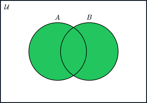
The standard way to picture a set is as a circle, with each circle drawn inside a rectangle standing for the universe $\mathcal{U}$. Whenever an operation includes some region formed by these circles, we shade that region green.

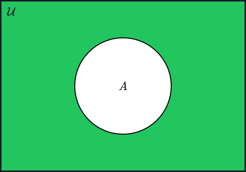
Complement

Since the complement of $A$ consists of everything in the universe that isn’t in $A$, the circle for $A$ itself is left unshaded, while everything else within the surrounding rectangle is shaded to represent $A^C$.

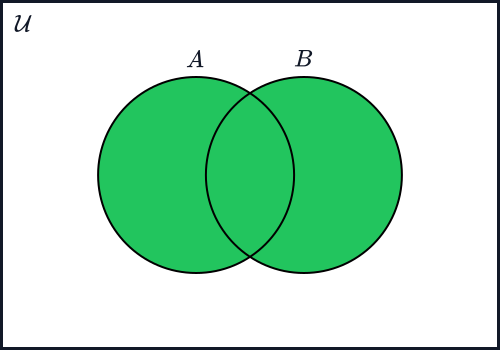
Union

As long as an element is in $A$ or $B$, or even both, it’s included in the union — so both circles are shaded in their entirety, overlap included.

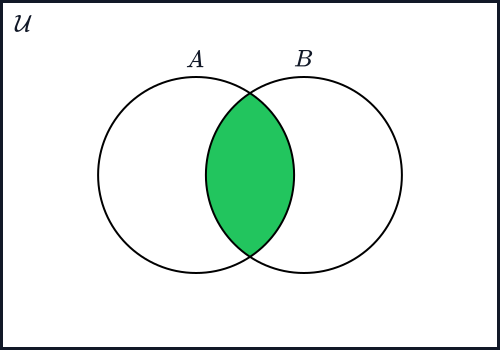
Intersection

Here, only the sliver shared by both circles is shaded, since that’s the only region representing elements common to both $A$ and $B$.

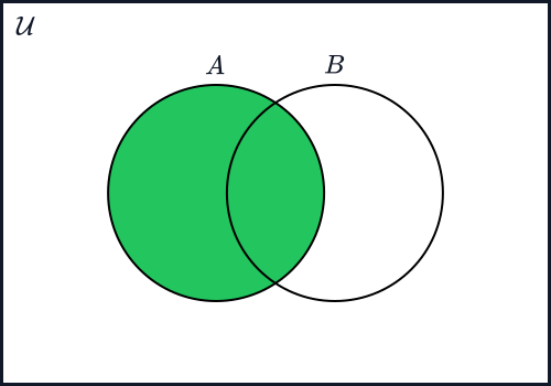
Difference

Only the part of $A$’s circle left over once the overlapping sliver shared with $B$ has been carved away is shaded.

Symmetric Difference

The symmetric difference shades everything covered by either circle except the overlapping sliver shared by both — everything a union would shade, minus whatever an intersection would shade.

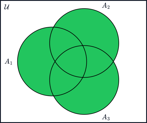
Multiple Union

This same idea of shading extends naturally to more than two sets at once — every region covered by at least one of $A_1$, $A_2$, or $A_3$ is shaded to represent their multiple union.

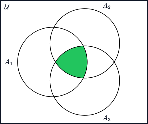
Multiple Intersection

Here, only the single region shared by all three circles at once — where $A_1$, $A_2$, and $A_3$ all overlap — is shaded, representing their multiple intersection.

The Laws of Set Theory

Understanding the laws of set theory is essential because they solve the problem of determining when two or more sets are equal, through fundamental equations including associativity, commutativity, and distribution. These laws provide a structured framework for defining and manipulating sets, ensuring consistency and precision in operations such as subset, difference, and symmetric difference.

In other words, by developing laws of set theory, we can essentially manipulate equations involving sets as if they were algebraic equations. In addition, the laws of set theory will allow us to convert complicated expressions involving sets into simpler ones, much like how we took complicated logical expressions and simplified them into smaller, logically equivalent expressions.

By studying these laws, one can formulate and prove mathematical concepts and theorems accurately. Furthermore, the foundations of many branches of mathematics are developed using the language of sets and set theory. In addition to the further development of mathematics, these laws also prove crucial to subjects like computer science and data science.

Equal Sets

We’ve briefly described some aspects of set equality when we first introduced what sets were. We talked about how repetition and order are irrelevant with respect to what elements are contained within a set. As such, even if some elements are repeated in various descriptions, they still represent the same set.

However, as we’ve also seen, there are a wide variety of methods to describe a set and what elements are contained within it. Just because we come up with different descriptions, that doesn’t necessarily mean we’re describing different sets — sometimes we may be describing exactly the same set.

However, defining set equality by having the same elements isn’t exactly rigorous. Two sets can share some number of elements while also having different elements. As such, we don’t define set equality by simply having the same elements — instead, we look to the end of the previous example for inspiration.

This definition is precise because we can determine whether a set is a subset of another set under scrutiny. As such, because the definition of set equality requires we show two things to be true, proofs showing two sets to be equal are usually broken up into two parts.

It’s this definition of set equality that makes the next two theorems somewhat straightforward to prove.

Thus, by this theorem, whenever we know that $A \subseteq B$, we can replace $A \cap B$ with just $A$ anywhere we see $A \subseteq B$ in an equation. It’s worth stressing that we can only make such a replacement when we know $A \subseteq B$ — otherwise, doing so may not be correct.

There are a few more such equalities we can make use of, which we now show in the next theorem.

Because of this theorem, whenever we know one of

is true, we automatically know that the other three are true as well.

Disjoint Sets

The total opposite of two sets $A$ and $B$ being equal is when $A$ and $B$ have absolutely no elements in common. Of course, if two sets share no element in common, then their intersection is a set with no elements in it — the empty set.

Many of the concepts discussed so far may seem disparate. However, they’re more connected than may initially appear.

This theorem connects the concepts of equal sets, disjoint sets, unions, and symmetric differences.

Membership Tables

Remember that $x \in A$ is a statement about $x$ being a member of set $A$. Because it’s a statement, it has a truth value of either $0$ or $1$.

One powerful tool we had at our disposal for analyzing logical expressions was a truth table. We can adapt truth tables to analyze set relationships as well. In this case, membership tables offer a tabular way of representing element arguments.

Instead of using some generic symbol for a generic object whose membership in some set we want to analyze, we could simply list whatever sets we’re analyzing. As such, we could rewrite the above table like so:

All of the set operations have their corresponding tables, which we can include inside one large table:

Based on the values above, we see that there are obvious analogues with logical operators:

Notice that the set difference resembles the logical complement of an implication.

In addition to the set operations, we can determine subset relationships. Let’s take a look at one more table to see an example:

Notice that the columns $(x \in A \cap B) \to (x \in A)$ and $(x \in A) \to (x \in A \cup B)$ have all $1$s. As such, we can write

which is exactly the definition of subset. As such, we can determine that a set $A$ is a subset of some other set $B$ by comparing their respective columns. If $A$ has $1$s in every row where $B$ also has a $1$, then we know that $A \subseteq B$.

Let’s prove a simple observation we may have had in our study of set relationships and operations.

Membership tables can be a convenient way to represent an element argument in tabular form. However, membership tables won’t totally replace element arguments, as sometimes the element argument is simpler to make for more esoteric situations where tables can be cumbersome to use.

Some Laws of Set Theory

We’ve already examined a number of simple laws (referred to as theorems) above, and have demonstrated their truth by way of element arguments and membership tables. What’s demonstrated above only scratches the surface of the multitude of equal-set relationships we can exploit. Below, we present a large table offering even more such laws.

As you look over this table, it would be wise to compare it with the table presented in Chapter 1, Section 5. You should see many analogues.

For any sets $A$, $B$, and $C$ taken from some universal set $\mathcal{U}$, we have the following equivalencies:

Certainly, many more such laws and equivalencies exist, but the table above represents some of the more ubiquitous laws that are often used.

These laws present us an opportunity to directly compare three different proof techniques. First, we use a membership table.

Now, compare such a simple strategy with a standard element argument used in the next proof.

The last of these laws we’ll prove in this section will be the Distributive Laws. Instead of making two separate element arguments to establish that $A \cup (B \cap C) \subseteq (A \cup B) \cap (A \cup C)$ and $(A \cup B) \cap (A \cup C) \subseteq A \cup (B \cap C)$, we’ll use logical equivalencies to show that $A \cup (B \cap C)$ and $(A \cup B) \cap (A \cup C)$ are subsets of each other simultaneously.

Of course, the rest of the Laws of Set Theory can be proven in many different ways. Because it’s a good exercise to provide a proof for all the above laws, proofs for the remaining laws are asked for in this chapter’s practice questions.

Using the Laws of Set Theory

Just as we can use the Laws of Logic to simplify complicated logical expressions, we can also use the Laws of Set Theory to simplify complicated expressions involving sets.

We made use of an additional law of Set Theory above, where we can express the set difference operation using only intersection and complement:

We’ll now justify that equality:

For any two sets $A$ and $B$ taken from some universal set $\mathcal{U}$, we have that

As a matter of fact, we can also express the symmetric difference operation using only union, intersection, and complement, which we justify below:

For any two sets $A$ and $B$ taken from some universal set $\mathcal{U}$, we have that

This just goes to show how important the union, intersection, and complement operations are when it comes to sets, because no matter how we want to combine any combination of sets, we can always do so using just those three operations.

Generalized DeMorgan’s Laws

We’ve seen DeMorgan’s Laws applied to two sets at a time. Let’s see what happens when we have three sets at a time:

It stands to reason that repeated applications of DeMorgan’s Laws would work for intersection as well.

Furthermore, no matter how many sets we have, it seems as if we can just repeatedly apply DeMorgan’s Laws and the Associative Law. Based on this observation, we make the following observations, where $I$ is an index set over which the multiple union or intersection is taken:

Of course, mere intuition doesn’t prove anything to be true. Instead, we must rely on rigorous tools, such as element arguments and logical equivalencies, to establish truth without any doubt.

The generalized versions of DeMorgan’s Laws will prove extremely useful in our further study of math.

Proof Technique: Exhaustion

All of the proof techniques discussed thus far work on sets that have infinitely many elements. For example, we’ve talked about theorems that apply to all even numbers, not merely some of them. For example, for all even numbers, adding one yields an odd number. As another example, no matter which two even numbers are added together, the sum is always another even number.

We’ve even talked about theorems that apply to all sets in general, not merely some of them. These include the set operations and the set equalities.

It’s not hard to see why methods that apply to sets of infinitely many objects are powerful. On the other hand, there may be times when there are only a finite number of objects we’re interested in examining. Here, we discuss a method for proving theorems dealing with only a finite number of elements.

A Contrived Example

Admittedly, dealing with only a finite number of elements seems hardly useful, as we mostly want results that apply generally, and not specifically. Here, we provide a contrived example simply to demonstrate the technique.

We could perhaps call the result derived in the previous example a theorem, since we did provide a proof for the fact, but we prefer to reserve the term theorem for “major” results. That result was merely an exercise.

The Method of Exhaustion

Based on the previous example, we can see why the method presented in this section is called the Method of Exhaustion: it’s because we exhaustively check every single element in the desired set for a desired property. Note that while the term exhaustion is used to describe the thoroughness of checking every element, it doesn’t necessarily refer to the feeling one may get whilst performing the checking — though it should be said that for rather large sets, this method can be tiresome.

Let’s lay out the argument in logical fashion, same as we’ve done before. The reason this method works is because we verify that every element in the desired set has some desired property.

Suppose set $A$ is a finite subset consisting of the $n$ elements

taken from some universal set $\mathcal{U}$. Furthermore, suppose $p$ is an open statement defined on $\mathcal{U}$. The Method of Exhaustion is simply an argument of the form

That’s all there really is to it.

Computer-Assisted Proofs and the Four Color Theorem

Just because a set is finite doesn’t mean it’s feasible to hand-check every single element within it. Sometimes tasks can be automated by writing computer programs to check thousands or even millions of elements in a timely fashion.

While the example presented above was rather contrived, one major result proved using the Method of Exhaustion was the Four Color Theorem. This theorem states that any planar (basically meaning flat) map only needs at most four different colors so that no adjacent regions on the map share the same color. For centuries, cartographers have been making maps of various places around the world, and one way to draw maps is to color regions so they’re easily distinguishable. It’s typically expected that adjacent regions on a map are colored differently, helping them stand out visually.

It was shown at some point in the late 1800s that no more than five colors were needed for any map so that no adjacent regions shared a color, but it was suspected that no more than four colors were needed as well. Though many mathematicians attempted to prove that no more than four colors were needed, many efforts proved fruitless.

Progress marched forward in the 1960s with the advent of computing technology. Two mathematicians, Kenneth Appel and Wolfgang Haken, further developed results derived from Heinrich Heesch to complete a proof. Essentially, one major step in the proof was showing that all maps could be “reduced” to a small number of essential configurations (basically, all maps are distortions of some simpler underlying map that represent the same types of regions). Appel and Haken found that there were only $1834$ such configurations.

Once Appel and Haken found these configurations, it was simply a matter of checking each and every one of them — using the Method of Exhaustion.

This proof was the first major proof to be verified by computer. As such, it was a controversial result: not all mathematicians readily accepted the proof, because it was hard and time-consuming for a human to check.

Nevertheless, the proof has mostly withstood scrutiny, with a minor error being corrected by Appel and Haken sometime in the late 1980s.

The point is that while the Method of Exhaustion may seem overly simple and contrived, being restricted to only finite sets instead of infinite sets, it’s still a valid proof technique that can come in handy.

Set Partitions

When working with a set of related objects, we may want to split that set up into smaller, more manageable sets.

For example, we may want to split up the integers based on parity: even integers, and odd integers. When dealing with the real numbers, we may want to split them up into three separate sets: the positive real numbers, the negative real numbers, and the number $0$. One more example may be the positive rational numbers, where we split them up based on how big they are — we may have all of the positive rational numbers less than $1$ in one set, and all of the positive rational numbers greater than or equal to $1$ in the other set.

No matter how we split up a set, we’ll want to make sure that all elements of the original set are accounted for in one of the smaller subsets we form.

Partitioning a Set

In the introduction to this section, we mentioned three examples of how we may split a large set into smaller subsets, making sure every element within the original set is in one of the subsets. A partition of a set creates these subsets while making sure that every element is accounted for; however, the word partition also invokes the idea of separation — no two subsets should share any elements. The following definition of partition offers something more precise.

Note that none of the sets in the partition can be empty. The whole point of forming a partition is to take elements from the original set and put them into a subset.

Examples of Partitions

Proof Technique: Casework

Previously, we talked about a proof technique where we examine every single element of a finite set. In a sense, we examined multiple cases, and verified some result for each of those cases. An exhaustive proof is a special kind of proof by casework.

Sometimes, we may have trouble demonstrating that some result holds for a set of elements. However, if we partition the set into groups that have their own special traits, and those traits make it easy to show the desired result holds, a proof by casework can be used to establish the desired result for the entire set.

The Underlying Argument

Suppose we were trying to prove a statement of the form

Suppose that we somehow knew that

If we knew how to show that

we would then have that

Thus, because $p = p_1 \lor p_2 \lor p_3 \lor \dots \lor p_n$, we would also have that $p \to c$ by extension.

This proof technique is simply an extension of the Rule of Proof by Cases:

as presented in Chapter 2, Section 6. Even though we could have discussed this proof technique in Chapter 2, we decided to hold off until partitions were discussed, because a lot of casework is done by considering elements from disjoint sets. However, when doing casework, it’s not important that elements from the universe of discourse are in only one subset of a partition.

Whether we form a partition of the universe, or we split the universe up into overlapping subsets, isn’t important. What’s important is that, once we have our desired subsets, every element is represented by at least one of those subsets.

Picking Arbitrary Elements from a Partition

When we partition a set, we split it into disjoint subsets where every element is accounted for in one of the subsets. We don’t have to form these subsets arbitrarily. Instead, we could take all elements from the original set that have some common property, and stick those elements into a subset. We can repeat this process until all elements are accounted for.

Then, from each of these subsets, we choose an arbitrary element. Then, whatever is true of that element will be true for all elements within that subset. In essence, we’re using the principles of Universal Specification and Universal Generalization, along with a partition, to prove a theorem.

Our first theorem will be a result about absolute values of real numbers. As a reminder, here’s the definition of absolute value of a real number.

An Example with Lots of Cases

Here, we’re going to discuss perfect squares and what kinds of numbers can be the units digits of perfect squares. Before we discuss the next theorem, let’s make some observations about the non-negative integers.

From the observations presented in the previous example, we see that any non-negative integer can be written as $10a + b$. This observation will help us in the upcoming theorem.

A Common Mistake

The most common error that can occur when doing a proof by cases is not accounting for every element in the universe being considered. It is essential that all the cases you consider account for every possible element.

It may seem like the previous example demonstrates that $n^2 \geq n$ for all integers. After all, we showed it was true for positive integers and negative integers. However, there’s one integer that’s neither positive nor negative, namely $0$. In this situation, since it’s only one integer left unaccounted for, we could simply compute $0^2$ and compare it to $0$ to determine that the above statement is indeed true for all integers. We formalize this proof now.

Russell's Paradox and a Formal Resolution

Sets are a powerful abstraction that allows us to collect a wide variety of objects into one structure. Typically, all objects within a set share some common characteristic other than mere inclusion in the set. They may be points on the plane, equilateral triangles, even numbers, or even fruits.

As powerful as sets are, we haven’t given a formal definition of what a set is. We’ve been relying on an intuitive definition, and though it works well enough for our purposes, sooner or later the cracks start to show. Sometime around 1901, a mathematician named Bertrand Russell formulated his now-infamous paradox that seemed to dismantle the entire theory of sets. The scary thing about the paradox is that a lot of mathematical research and important results rested on the foundations of Set Theory. If Set Theory is wrong, are all results depending on sets wrong as well?

In this section, we’ll eke out what this paradox is, and hint at a solution that solves the problem.

Sets That Are Members of Other Sets

Over the course of this chapter, we’ve defined sets that mostly have numbers, though we’ve constructed other more intricate sets. Sometimes we’ve constructed sets that contain other sets.

We’ve got a handle on this situation, but let’s ask a more interesting question:

Can a Set Contain Itself?

What would it look like for a set to contain itself? Let’s see if we can make such a set.

Determining if a set is contained in another set when both sets contain infinitely many elements takes some care, so we’ll sidestep that issue by considering the following set:

What kind of set is $\boxtimes$? It’s a set whose elements are sets. But these are special sets. In the previous example, we were concerned with what a set that contains itself would look like. Here, we don’t scrutinize whether a given set contains itself. Instead we’re just assuming that we’ve somehow curated every set, and are only including sets that don’t contain themselves.

Now consider the following question: is $\boxtimes$ contained within $\boxtimes$? Remember that for propositions such as $\boxtimes \in \boxtimes$, there are only two possibilities: either $\boxtimes \in \boxtimes = 0$ or $\boxtimes \in \boxtimes = 1$. Let’s consider both possibilities.

Case 1: $\boxtimes \in \boxtimes = 0$.

Here, we’re considering the possibility where $\boxtimes$ doesn’t contain itself. Well, since $\boxtimes \notin \boxtimes$, we know that

However, notice what the logical implications are if $\boxtimes \notin \boxtimes$: either $\boxtimes$ is not a set (it is, so this would be a contradiction) or $\boxtimes \in \boxtimes$ (which contradicts the supposition that $\boxtimes \notin \boxtimes$). Either way, the proposition $\boxtimes \notin \boxtimes$ yields contradictions. As such, we may suspect that $\boxtimes \in \boxtimes = 1$. Let’s check.

Case 2: $\boxtimes \in \boxtimes = 1$.

Suppose we somehow knew that $\boxtimes \in \boxtimes$.

So, by assuming $\boxtimes \in \boxtimes$, the logical implication is that $\boxtimes \notin \boxtimes$? This is a clear contradiction.

At this point, both cases yield contradictions. This could be a problem, but solutions do exist.

Resolving the Paradox

How come we haven’t had this problem dealing with any of the previously defined sets in this chapter? It has to do with the fact that we were constructing sets with particular objects. Even numbers are easy to grasp, quadrilaterals are easy to grasp, but abstract set requirements aren’t so easy to grasp. We even had trouble trying to come up with a set that contained itself in the second example above.

While not a resolution to the paradox, defining sets using easy-to-grasp elements does at least avoid the issue.

Perhaps the most commonly used formal system of Set Theory is ZFC Set Theory. ZFC is short for Zermelo–Fraenkel–Choice, where Zermelo and Fraenkel are the two mathematicians who formulated this type of Set Theory, and the word choice refers to the Axiom of Choice, which is something that will be examined later in this book.

ZFC Set Theory came around in the early 20th century, and is free of paradoxes like Russell’s Paradox. ZFC Set Theory is an intricate system, and requires some more advanced mathematics to understand. While it isn’t discussed in this book, further reading on ZFC Set Theory and on the history of Russell’s Paradox is easy to find, for anyone curious enough to look into how it inspired the search for more axiomatic systems of Set Theory.