In most mathematics courses a student has taken so far, they have usually
been presented with a collection of results — facts they can use whenever
warranted. Polynomials, for instance, come with a wide variety of such
facts: how to divide one polynomial by another, how to find the roots of a
quadratic equation, and so on.
Geometry offers just as many. The Angle Bisector Theorem tells us that the
bisector of an angle in a triangle divides the opposite side into two
segments proportional to the triangle’s other two sides. A wide variety of
theorems describe the chords of a circle. And the famous Pythagorean
Theorem relates the three sides of a right triangle.
At some point, a student may wonder why these results are true — how do we
know for certain they’re correct, rather than simply guesses that happen to
look accurate? The answer is that we use a system of logic to rigorously
prove, beyond any doubt, that such results are true rather than mere
guesses. With a system of logic in hand, we no longer have to wonder
whether the results we’ve come to rely on are mystical in nature, handed
down on stone tablets — they are results we can work out ourselves, with
infinite precision.
Over the next two chapters, we build up a system of logic that lets us
derive the truth of many of the results we’ve already seen, along with
results yet to come.
Subsections of Logic
Propositions
In Mathematics, we deal with statements like these:
\[
\begin{align*}
&\text{Squares have four equal sides.} \\
\\
&\text{Quadratic equations have at most two} \\
&\text{distinct roots.}
\end{align*}
\]
In life, we deal with statements like these:
\[
\begin{align*}
&\text{If you don't pay your parking tickets, then} \\
&\text{you will go to jail.} \\
\\
&\text{The rent was paid on the first of the month, and the} \\
&\text{air conditioner stopped working.}
\end{align*}
\]
In Math, as in life, some statements are easy to determine if they’re true
or false. However, when we encounter more complicated expressions, we
typically need a way to carefully evaluate that statement’s truth.
We can start to evaluate these expressions by examining simple expressions,
then simple combinations of expressions, and working our way up, so to
speak, to increasingly more complicated expressions until we finally have
the truth of the desired expression.
In this section, we talk about how to evaluate these simple expressions,
and how to combine those simple expressions.
Defining Propositions
We start by defining what a proposition is:
PROPOSITION, STATEMENT
A proposition is a declarative sentence that is either true or false.
We also often use the term statement to describe such a sentence.
Propositions are the building blocks of any logical system. These are what
we evaluate and combine to form larger statements.
Example 1.1.1: Some examples of propositions
\[
\begin{array}{rl}
w\text{: } &\text{H}_2\text{O is a liquid at 70 degrees Fahrenheit and 1 atmosphere.} \\
t\text{: } &\text{Mr. T was a mathematics major at Prairie View A\&M University.} \\
j\text{: } &\text{Thomas Jefferson was the second president of the United States.} \\
b\text{: } &\text{Mary Shelley wrote Frankenstein or Alexandre Dumas wrote Moby Dick.} \\
x\text{: } &\text{12 is divisible by 3.} \\
y\text{: } &\text{3 + 3 = 7 and 4 + 4 = 8.} \\
z\text{: } &\text{2 is a solution to the equation } z^2 - 4 = 0 \text{.}
\end{array}
\]
As a convention, we often use lowercase letters to refer to specific
propositions we are working with.
All of the sentences in the previous example have definite truth values.
Example 1.1.2: Looking at the truth values of the previous examples
\[
\begin{array}{rll}
w\text{: } &\text{H}_2\text{O is a liquid at 70 degrees Fahrenheit and 1 atmosphere.} &\text{(true)} \\
t\text{: } &\text{Mr. T was a mathematics major at Prairie View A\&M University.} &\text{(true)} \\
j\text{: } &\text{Thomas Jefferson was the second president of the United States.} &\text{(false)} \\
b\text{: } &\text{Mary Shelley wrote Frankenstein or Alexandre Dumas wrote Moby Dick.} &\text{(true)} \\
x\text{: } &\text{12 is divisible by 3.} &\text{(true)} \\
y\text{: } &\text{3 + 3 = 7 and 4 + 4 = 8.} &\text{(false)} \\
z\text{: } &\text{2 is a solution to the equation } z^2 - 4 = 0 \text{.} &\text{(true)}
\end{array}
\]
Compound Propositions
You’ll notice that some of the propositions in the previous examples look
like they consist of simpler propositions.
Example 1.1.3: Breaking complex propositions into simple propositions
Proposition $b$ from the previous two examples is made up of two simpler propositions:
\[
\begin{array}{rll}
b_1\text{: } &\text{Mary Shelley wrote Frankenstein.} &\text{(true)} \\
b_2\text{: } &\text{Alexandre Dumas wrote Moby Dick.} &\text{(false)}
\end{array}
\]
Proposition $y$ from the previous two examples is also made up of simpler propositions:
Notice that there really isn’t a way to break up propositions $b_1$, $b_2$,
$y_1$, $y_2$ into anything simpler.
Some propositions can be broken up into simpler propositions. Other
propositions are already expressing a simple claim that isn’t a
combination of other simple claims.
PRIMITIVE PROPOSITION, COMPOUND PROPOSITION
A primitive proposition is a proposition that expresses a simple claim
that cannot be decomposed into any simpler propositions.
A compound proposition is a proposition that is made by combining
simpler propositions together.
Note that the above definition of a compound proposition does not require
its constituent propositions to themselves be primitive — any combination
of primitive and compound propositions can be combined to form one larger
compound proposition.
There are a large number of ways we can combine propositions, primitive or
compound, together to form more complicated propositions.
Logical Connectives
We start by introducing a very simple way to make a more complicated
proposition from a single proposition.
NEGATION
The negation of a single proposition $p$, denoted $\neg p$, has a truth
value that is opposite of the truth value of $p$.
That is to say, if $p$ is true, then $\neg p$ is false. If $p$ is false,
then $\neg p$ is true.
We do not consider the negation $\lnot p$ of a proposition $p$ to be primitive.
The rest of the logical connectives we introduce combine two given
propositions into one proposition.
CONJUNCTION
The conjunction of two given propositions $p$ and $q$, denoted
$p \land q$, is true when $p$ and $q$ are both true. Otherwise,
$p \land q$ is false.
DISJUNCTION
The disjunction of two given propositions $p$ and $q$, denoted
$p \lor q$, is true when at least one of $p$ or $q$ is true. Otherwise,
$p \lor q$ is false.
Note that in this definition, or is true when both propositions in the disjunction are also true. Usually in spoken and written English, or is used in an
exclusive sense, meaning only one of the propositions is true. In Mathematics, or is almost always taken to be inclusive, and will be the case throughout the
rest of these notes. Unless otherwise stated, you should assume the word or is being used inclusively.
The following logical connective more closely aligns with what most people normally say when they use the word or.
EXCLUSIVE-OR
The exclusive-or of two given propositions $p$ and $q$, denoted
$p \veebar q$, is true when exactly one of $p$ or $q$ is true. Otherwise,
$p \veebar q$ is false.
The next definitions have to do with cause-and-effect type relationships between two propositions.
IMPLICATION, CONDITIONAL
The implication of two given propositions $p$ and $q$, denoted
$p \to q$, is false when $p$ is true and $q$ is false.
Otherwise, $p \to q$ is true.
An implication is also called a conditional.
BICONDITIONAL
The biconditional of two given propositions $p$ and $q$, denoted
$p \leftrightarrow q$, is true when $p$ and $q$ have the same truth
value — that is, when $p$ and $q$ are both true, or both false. Otherwise,
$p \leftrightarrow q$ is false.
Translating Compound Propositions into English Sentences
Knowing how the truth value of a compound proposition relates to the truth values of its constituent propositions will provide
guidance on how to translate a symbolic logical expression into familiar English sentences.
For starters, note that since $\neg p$ has the opposite truth value of $p$, we can describe the truth value of $\neg p$ as not whatever
$p$ happens to be since $\neg p$ can only be true or false. As such, we usually translate $\neg p$ as “Not $p$”.
Next, by our definition of conjunction, we know that a compound proposition such as $p \land q$ is true only when $p$ and $q$ are both
true. Hence, we translate the symbolic expression $p \land q$ as “$p$ and $q$”.
Since the mathematical definition of disjunction is inclusive, we can (or probably should) translate the symbolic expression $p \lor q$ as
“$p$ or $q$, or both” in order to emphasize the inclusive nature of disjunction. Again, based on the definition though, it should be understood
that the sentence “$p$ or $q$” is the inclusive version of the word or.
On the other hand, for the exclusive-or, we do need to indicate in the English sentence that not both must be true. This means when we translate
an expression such as $p \veebar q$, we do need to translate this roughly as “$p$, or $q$, but not both”, or perhaps something similar indicating
only one of the propositions is true.
The implication is perhaps the most complex expression to translate into English. We won’t be able to start appreciating why this is until
Chapter 2, but note that there are a wide variety of ways we can translate an implication into English. Some of these translations may seem confusing now,
but should become clear the more we work with implications (again, a detailed discussion of implications will be postponed to Chapter 2). For now,
here is a large list of possible translations for the logical expression $p \to q$:
“If $p$, then $q$”
“$p$ implies $q$”
“$p$ is sufficient for $q$”
“$p$ is a sufficient condition for $q$”
“$q$ is necessary for $p$”
“$q$ is a necessary condition for $p$”
“$p$ only if $q$”
“$q$ if $p$”
“$q$ whenever $p$”
Likewise, the biconditional can also be a bit cumbersome, but we will examine the biconditional in large detail in the upcoming sections. For now,
here is a list of ways the biconditional $p \leftrightarrow q$ can be translated into English:
“$p$ if and only if $q$”
“$p$ is necessary and sufficient for $q$”
Of course, there may be more elegant ways to translate propositions into English sentences. Having some command over the language gives you more ability
to translate these into English sentences, but the above methods more than suffice in most instances.
Example 1.1.4: Combining propositions into compound propositions
Consider the following propositions (disregarding for now whether they are
true or not):
\[
\begin{array}{rl}
i\text{: } &\text{Aliens Florp and Flarp invade Earth.} \\
f\text{: } &\text{The flying saucer has plenty of plutonium based fuel.} \\
t\text{: } &\text{The flying saucer has enough capacity to store and transport three Earth specimens.} \\
s\text{: } &\text{Florp and Flarp's invasion of Earth is successful.}
\end{array}
\]
Now we translate each of the following logical expressions into English
sentences:
$\neg f$
$$\text{The flying saucer is not stocked with plenty of plutonium-based fuel.}$$
$t \land \neg i$
\[
\begin{align*}
&\text{The flying saucer has enough capacity to store and transport three Earth specimens, and} \\
&\text{Aliens Florp and Flarp do not invade Earth.}
\end{align*}
\]
$f \lor \neg s$
\[
\begin{align*}
&\text{The flying saucer is stocked with plenty of plutonium-based fuel, or} \\
&\text{Florp and Flarp's invasion of Earth is not successful.}
\end{align*}
\]
$f \veebar t$
\[
\begin{align*}
&\text{Either the flying saucer is stocked with plenty of plutonium-based fuel, or} \\
&\text{it has enough capacity to store and transport three Earth specimens,} \\
&\text{but not both}
\end{align*}
\]
$\neg f \to \neg i$
\[
\begin{align*}
&\text{If the flying saucer is not stocked with plenty of plutonium-based fuel, then} \\
&\text{Aliens Florp and Flarp do not invade Earth.}
\end{align*}
\]
$t \to s$
\[
\begin{align*}
&\text{If the flying saucer has enough capacity to store and transport three Earth specimens, then} \\
&\text{Florp and Flarp's invasion of Earth is successful.}
\end{align*}
\]
$f \leftrightarrow i$
\[
\begin{align*}
&\text{The flying saucer is stocked with plenty of plutonium-based fuel if and only if} \\
&\text{Aliens Florp and Flarp invade Earth.}
\end{align*}
\]
Sentences That Are Not Propositions
Of course, not all sentences represent propositions. A sentence is only a proposition if it is true or false (but not both). Any sentence
that can’t be described as true or false is not a proposition.
Example 1.1.5: Sentences that do not represent propositions
“What time is it?” This is a question, not a declarative sentence, so it
can’t be assigned a truth value.
“File your taxes before April 15.” This is a command, not a declarative
sentence — it tells someone to do something rather than asserting a fact
that is true or false.
“$x + 3 = 10$.” Whether this sentence is true or false depends on the
value of $x$, which we don’t know, so we can’t determine its truth
value.
“What a gorgeous sunset!” This is an exclamation expressing an opinion,
not a statement of fact with a definite truth value.
“This statement is false.” This is a self-referential statement. Assuming the statement is true means the
statement is false. Assuming the statement is false means it is true. There is no consistent truth value
for this sentence, and as such, means it is not a proposition.
Modeling Logic with Truth Tables
We are often working with three or more propositions at a time, usually
combined into large numbers of expressions made using the logical
connectives discussed previously.
It can be cumbersome to work with them individually. Here, we will learn a
technique for handling multiple expressions efficiently.
A Convenient Shorthand
To make our upcoming work easier, we adopt a common shorthand for truth
values:
Using numbers will make the following concept a bit more space efficient,
and give a more mathematical flavor going forward.
Atomic Propositions: Building Blocks of Truth Tables
A truth table is simply a table organizing multiple logical expressions
based on the truth values of their constituent, or atomic propositions.
By atomic, we mean propositions used to construct compound propositions
by combining them with logical connectives.
In the expressions
\[
\begin{align*}
& \neg p \\
& p \land q \\
& p \lor q \\
& p \veebar q \\
& p \to q \\
& p \leftrightarrow q
\end{align*}
\]
$p$ and $q$ are considered atomic.
Note that atomic propositions themselves do not need to be primitive.
Example 1.2.1: Identifying atomic propositions in logical expressions
Let $p$ and $q$ be compound propositions defined as follows:
\[
\begin{array}{rl}
p\text{: } &a \land b \\
q\text{: } &a \lor b
\end{array}
\]
In the context above, $a$ and $b$ are the atomic propositions.
Now reconsider the six expressions from earlier:
$\neg p$
$p \land q$
$p \lor q$
$p \veebar q$
$p \to q$
$p \leftrightarrow q$
Here in these expressions, $p$ and $q$ are also considered atomic, since
they are named propositions being connected together to form compound
propositions. We could go a step further and substitute in the definitions
of $p$ and $q$ given above, in terms of the propositions $a$ and $b$:
$\neg (a \land b)$
$(a \land b) \land (a \lor b)$
$(a \land b) \lor (a \lor b)$
$(a \land b) \veebar (a \lor b)$
$(a \land b) \to (a \lor b)$
$(a \land b) \leftrightarrow (a \lor b)$
In general, a proposition that is named or labeled (usually with a
lowercase letter) is considered atomic because it can be used to build up
other propositions when combined with other labeled propositions using the
logical conenctives.
Constructing Truth Tables
As stated before, a truth table is simply a table showing the truth value
of a logical expression based on the truth values of its atomic
propositions.
Here is an overview:
We start with the given expression, and identify all atomic propositions
used to form it.
We create a table with enough columns for all of the atomic propositions
as well as the desired logical expression. We list all atomic
propositions in the left-most columns, in alphabetical order. The last,
right-most column is reserved for the desired proposition.
Under the columns for the atomic propositions, we list all possible
combinations of truth values between the atomic propositions. A good way
to ensure that all combinations are listed is to follow a “rotary,”
“dial,” or “odometer” method, where the right-most atomic proposition’s
values change the most frequently between rows, and the first,
left-most atomic proposition’s values cycle the least frequently between
rows. Instead of dialing through digits 0 through 9 like an odometer,
you flip back to 0 after reaching 1.
For each row, evaluate the desired logical expression by substituting
that row’s truth values in for its atomic propositions.
This yields a complete truth table for your desired expression. Let’s see
an example where we fill out a truth table for the logical expression
$p \land q$:
Example 1.2.2: Constructing a truth table for $p \land q$
Step 1: Identify the atomic propositions
For $p \land q$, the atomic propositions are $p$ and $q$.
Step 2: Create an initial table that has enough columns to hold the atomic propositions and the desired proposition
There are two atomic propositions, along with the desired proposition, so
our table needs three columns: $p$, $q$, and $p \land q$. We list the
atomic propositions first, in alphabetical order, and then end with the
desired proposition.
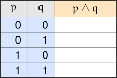
Step 3: List all possible combinations of truth values for the atomic propositions being used
Here is what the overall table’s structure will look like. In this book, we will use a
blue color to color in all of the values for the atomic propositions, and
an orange color for the desired expression’s column.
Examine the way the truth values for the atomic propositions have been laid
out. As described earlier in the overview, we are listing each combination
of truth values by essentially using a rotary or dial system. This ensures
we list all possible combinations of truth values.
Step 4: Fill in all of the missing truth values under the desired proposition’s column
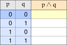
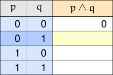
Let’s do this one row at a time. Let’s start with the first row, where
$p = 0$ and $q = 0$, highlighted in this table:
What value do we fill in to the highlighted, yellow cell? We need to refer
back to the definition of conjunction: the conjunction of two propositions
$p$ and $q$, denoted $p \land q$, is true only when both $p$ and $q$ are
true. If either $p$ or $q$ is false, then the conjunction itself is false.
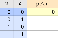
Remember that we use $0$ to represent a false truth value, and $1$ to
represent a true one. In the row we’re examining, both $p$ and $q$ are
false, since both are equal to $0$. Since not both $p$ and $q$ are true,
$p \land q$ is false, so we write $0$ in the highlighted cell, as shown
below:
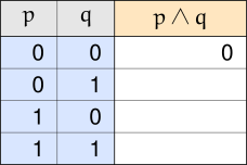
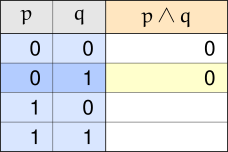
This leaves us with the following partially filled out table:
We continue on to the next row, where $p = 0$ and $q = 1$, highlighted
below:
Appealing to the definition, since one of the atomic propositions is
false — here, $p = 0$ — the conjunction $p \land q$ is also false. We place
a $0$ in the highlighted cell, shown below:
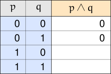
This leaves us with a slightly more filled out table, shown below:
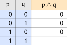
Let’s continue on and examine the third row, where $p = 1$ and $q = 0$.
Here, since one of the atomic propositions is false, the conjunction
$p \land q$ continues to be false, and we fill in a $0$ in the third blank
cell, shown below:
Now we are on the last row, where $p = 1$ and $q = 1$. Here, both atomic
propositions are true. This means the conjunction $p \land q$ is, by
definition, true. That means in this final blank cell we fill in a $1$,
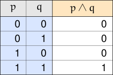
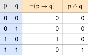
leaving us with the completed truth table for the conjunction $p \land q$:
This example shows the basic procedure. From now on, we can just fill in
the values as needed, without any need to repeat any of the exposition
here.
Truth Tables for the Logical Connectives
We have seen how to construct a truth table from scratch. Now, it’s really
just a matter of appealing to the definitions of the logical connectives in
order to construct truth tables for them. Knowing the truth tables for the
logical connectives is going to make working with even more complicated
expressions much easier, since any complicated expression is essentially
just a bunch of atomic propositions combined with the logical connectives
described here.
Here, we are going to use $p$ and $q$ as the atomic propositions for the
expressions.
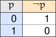
Negation $\neg$
This is a really simple truth table, since negation can operate on one
proposition at a time. Remember that the negation of a proposition has the
opposite truth value of the proposition itself.
Conjunction $\land$
We already saw this in the example above, but we’ll show the table here
for the sake of completeness.
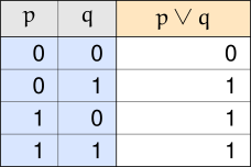
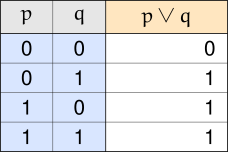
Disjunction $\lor$
Based on the definition of disjunction, we know that if at least one of the
atomic propositions is true, then the disjunction itself is also true.
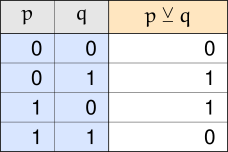
Exclusive-or $\veebar$
The definition essentially tells us that the exclusive-or of two atomic
propositions is true whenever the atomic propositions have different truth
values; or put another way, not equal to each other.
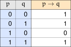
Implication $\to$
The definition of implication tells us that the only time an
implication is false is if $p$ is true, and $q$ is
false. Otherwise, the implication is true.
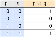
Biconditional $\leftrightarrow$
The definition for a biconditional essentially tells us that if the two
atomic propositions have the same truth value, meaning they are equal to
each other, then the biconditional itself is true. It is false otherwise.
We can almost think of the biconditional as being the exact opposite of an
exclusive-or between two propositions.
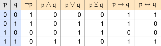
Combining All Logical Connectives Into One Table
Something we can do is simply append the columns for each of the logical
connectives into one big overall table. You have to be careful when doing
this to make sure the rows line up with the appropriate rows for the
atomic propositions. If the order of the atomic propositions differs, or if
the numbering method used yields a different ordering for the combinations
of truth values for the atomic propositions, the results may not be
correct.
Here, we used the same ordering for the atomic propositions themselves,
and the combinations of truth values for those atomic propositions. We
will have to extend the negation table by an additional two rows, but
again, we fill in any values needed by appealing to the definition of
negation, and paying attention to the values of the atomic propositions in
the row we are evaluating.
Intermediary Columns
Notice that we just produced a truth table that has more than one
expression column, one expression column for each of the logical
connectives we use to form compound propositions.
If we are trying to determine the truth value of a complicated expression,
we can do the same thing. We can identify all of the parts of the more
complicated expression, and gradually build up the truth value of the
final, desired expression. Doing this helps us keep track of values,
preventing us from having to work out complicated expressions all at once.
We use so-called intermediary columns to hold the parts of the
complicated expression that are easy to calculate. Usually, we break a
complicated expression up based on where the logical connectives are. Here
is an example.
Example 1.2.3: Using intermediary columns to construct a complicated truth table
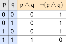
Consider the expression $\neg (p \land q)$. Working out its truth value
directly, row by row, means checking $p$, checking $q$, combining them with
conjunction, and then negating the result — three things to keep in your
head at once for every row.
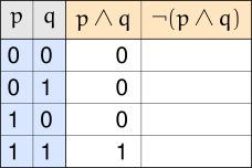
An intermediary column makes this easier. We start by building a table
with an intermediary column for the simpler piece, $p \land q$ — a table we
already know how to construct — alongside the column for the desired
expression $\neg (p \land q)$ itself, still blank:
To fill in that blank column, we no longer need to think about $p$ and $q$
at all — we just take the negation of whatever is already in the
$p \land q$ column, one row at a time:
All we need to do now is copy the Result column from the above table into the truth table we are building.
That’s the advantage of an intermediary column: instead of working out
$p$, $q$, and the negation of their conjunction all at once, we break the
work into two simple steps, each of which is just a single connective’s
truth table.
Example 1.2.4: A truth table for another complicated expression
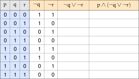
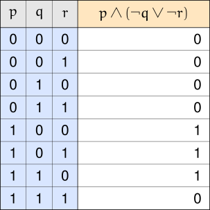
Consider the expression $p \land (\neg q \lor \neg r)$. This one has three
atomic propositions — $p$, $q$, and $r$ — so its full truth table needs
eight rows, and this time we’ll use more than one intermediary column.
We start with intermediary columns for the two simplest pieces, $\neg q$
and $\neg r$:
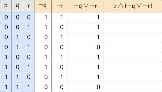
With those two columns in hand, we build a third intermediary column for
$\neg q \lor \neg r$, taking the disjunction of the two columns we just
built, row by row:
All we need to do now is copy the Result column from the above table into the truth table we are building.
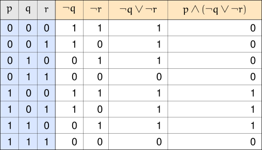
Finally, filling in $p \land (\neg q \lor \neg r)$ is just a matter of
taking the conjunction of $p$ column with the $\neg q \lor \neg r$ column we just
finished — no need to think about $q$ or $r$ individually at all:
We then copy the Result column from the above table into the truth table we are building, same as usual.
We could leave the table as it is, with a column for every intermediary
piece we used along the way. Or, we could construct a condensed table that
only shows the atomic propositions along with the desired expression.
Logical Order of Operations
Just like in the arithmetic of real numbers, there is an order we should
follow when evaluating logical expressions.
For instance, in the arithmetic of real numbers, we abide by the following
rules:
Parentheses $()$
Exponents
Multiplication and division (left to right)
Addition and subtraction (left to right)
Using this scheme for evaluating arithmetic expressions, we do the
following:
If we wanted to evaluate the disjunction first, we’d have to use
parentheses, since
$$p \land (q \lor r)$$
is not equivalent to the expression $p \land q \lor r$.
Using the Order of Operations
With the order of operations, we remove any ambiguity, and do not have to
rely on parentheses unless we want to give precedence to operations lower
in the order.
The final simplification reveals the final, overall truth value to be $0$.
A Note on Conventions
In this book, we adopt the above order of operations, but will only make
shallow use of it. Basically, what this effectively means is that we will
make very liberal use of parentheses, even when they aren’t strictly
necessary.
While the relative order between $\neg$, $\land$, $\lor$, $\to$,
and $\leftrightarrow$ is somewhat standardized (heavy emphasis on the
word “somewhat”), it is hardly universal. This is especially true when
$\veebar$ is thrown into the mix.
Many texts use $()$ liberally as well. In some ways, the
order of operations presented here was entirely engineered to meet this
book’s needs, and this order’s scope is only contained within this book.
This is why, going forward, we will hardly rely on this order of
operations, and instead opt to use the standard trick of using $()$ to
indicate which operations take precedence over others.
A Note on Organizing Arithmetic
A blank piece of paper allows one to express an idea anywhere on the page,
in any arrangement. But following a chain of arithmetic is much easier when
it’s laid out in a consistent, organized manner.
In this book, any arithmetic (based on real numbers, logic, or some other
system) will generally be shown in a tabular format. There will be two
benefits to this:
Relatively easy to follow from one step to the next.
Justification for each step can be explicitly shown.
Let’s see an example.
Example 1.3.4: Re-evaluating a complicated expression
We’ve seen plenty of primitive propositions whose truth values are fixed:
\[
\begin{array}{ll}
\text{Calvin Coolidge was the 30th President of the United States of America.} & \text{(true)} \\ \\
\text{Mitochondria convert ADP into ATP via cellular respiration.} & \text{(true)} \\ \\
\text{Leonardo da Vinci painted the famous ceiling fresco in the Sistine Chapel.} & \text{(false)}
\end{array}
\]
We’ve also seen compound propositions whose truth values depend on the
truth values of its atomic propositions.
\[
\begin{array}{ll}
2+2=5 \text{ and } 2+3=6. & \text{(false)} \\ \\
\text{Parallelograms with four equal sides and four equal angles are squares.} & \text{(true)} \\ \\
\text{If an integer is prime and even, then that integer is two.} & \text{(true)} \\ \\
\text{If } x=2 \text{ or } x=3 \text{, then } x^2-5x+6=0. & \text{(true)}
\end{array}
\]
Typically, the compound propositions we work with are made up of generic
propositions that could be true, or could be false. This means we
need to examine all combinations of truth values for the atomic
propositions to determine the overall truth value of the compound proposition.
Of course, we usually will only be interested in compound propositions
that are true. This is how we frame the upcoming discussion: when are compound propositions true?
Propositions that are Sometimes True
We’ve seen some examples of compound propositions that — for some
combinations of truth values — are true.
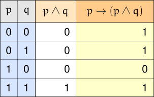
Example 1.4.1: Evaluating $p \to (p \land q)$
We construct a truth table. We’ll highlight the column we are interested in examining.
Only some of the combinations of truth values for $p$ and $q$ yield a
truth value of $1$ when combined in the desired compound proposition.
Those combinations are as follows: $p=0,q=0$; $p=0,q=1$; and $p=1,q=1$.
Only one combination yields a false truth value ($0$) when combined:
$p=1,q=0$.
Let’s dispense with the suspense; we already know what word we’ll use to
describe compound propositions that can be true.
SATISFIABLE
A compound proposition is called satisfiable if there exists some
combination of truth values for its atomic propositions that yield a
truth value of $1$.
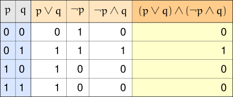
Example 1.4.2: Evaluating $(p \lor q) \land (\neg p \land q)$
Here, we see that there is only one combination of truth values for $p$
and $q$ for where $(p \lor q) \land (\neg p \land q)$ is true, namely
$p=0,q=1$.
Hence, $(p \lor q) \land (\neg p \land q)$ is satisfiable, even if just
barely.
Propositions that are Always True
We have yet to see a proposition that is always true, no matter what
combination of truth values are assigned to its atomic propositions.
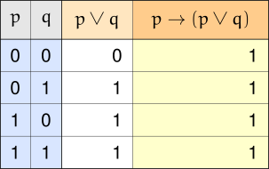
Example 1.4.3: Evaluating $p \to (p \lor q)$
We’ve seen $p \to (p \land q)$ above, but changing to the disjunction
yields interesting changes.
Notice that every row in the final column contains $1$.
TAUTOLOGY
A compound proposition is called a tautology when it is always true,
no matter what truth values are taken by its atomic propositions.
Sometimes when we come across a tautology in an expression, we can
replace it with the symbol $\top$ (sometimes also written $T_0$), but
since the truth value is always $1$, we can always replace the expression
with its truth value $1$.
It should be noted that it may preferable to either use $\top$ or $T_0$ when working with
propositions, because those symbols have additional context to them than the literal value $1$. Those
symbols signify that we are working with a proposition always happens to be true.
Propositions that are Never True
We’ve seen a proposition that is always true, but are there propositions
that are never true?
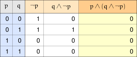
Example 1.4.4: Evaluating $p \land (q \land \neg p)$
Of course, we should probably expect this proposition to always be
false, because it is asserting both $p$ and $\neg p$.
You can’t assert both $p$ and $\neg p$, because they contradict each
other — which leads us to our next definition.
CONTRADICTION
A compound proposition is a contradiction when it is always false, no
matter what truth values are assumed by its atomic propositions.
Just like with tautologies, we sometimes use the symbol $\bot$ (sometimes
also written $F_0$) to represent a contradiction. But since a
contradiction is always false, we can also just use $0$ — though we may
prefer $\bot$ or $F_0$ if we wish to convey that we’re talking about a
proposition, rather than a literal value.
Laws of Logic
At this point, we’re familiar with the fundamental unit of logic — the
proposition. We’ve seen how to combine them into compound propositions,
and how to use truth tables to identify propositions that are always
true — tautologies.
With these tools, we are ready to start discussing the heart of logical
deduction and our unique ability to reason — the Laws of Logic!
A Simple Example
Before we dive into the deep end, let’s wade in a shallow example where we
examine a few propositions that involve the biconditional connective.
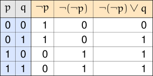
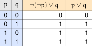
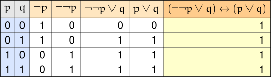
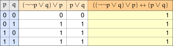
Example 1.5.5: Examining $\neg(\neg p) \lor q$
As usual, we can construct a truth table showing all intermediary values.
The final column resembles the truth table for the compound proposition
$p \lor q$:
So under all the exact same circumstances (meaning, same combinations of
truth values for $p$ and $q$) the expressions $\neg (\neg p) \lor q$ and
$p \lor q$ have the same truth value.
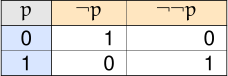
Let’s examine the double negation more closely:
We see that $p$ and $\neg \neg p$ have the exact same truth values,
regardless of what value $p$ has.
Since $p$ and $\neg \neg p$ always have the same truth values under all
conditions, we can swap them out with each other in expressions, without
affecting the overall truth value.
This explains why $\neg \neg p \lor q$ and $p \lor q$ have the same truth
values for all combinations of truth values for $p$ and $q$; because we
can swap out $\neg \neg p$ with just $p$ without affecting the truth
values.
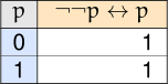
Notice that because $\neg \neg p$ and $p$ have the same truth values, we
expect the biconditional connecting them to always be true — a tautology:
\[
\begin{array}{l|l|l|l|l}
p & \neg p & \neg \neg p & \neg \neg p \leftrightarrow p & \text{Result} \\
\hline
0 & 1 & 0 & (0) \leftrightarrow (0) & 1 \\
1 & 0 & 1 & (1) \leftrightarrow (1) & 1
\end{array}
\]
It is as expected:
Furthermore,
So we see that $(\neg \neg p \lor q) \leftrightarrow (p \lor q)$ is a
tautology. We prefer $p \lor q$, since it’s a simpler expression than
$\neg \neg p \lor q$.
In the previous example we saw how — when the biconditional between two
propositions is a tautology — we can essentially just swap out one
expression that has the same behavior under its atomic propositions for
another, without changing the overall truth value.
Let’s see another example.
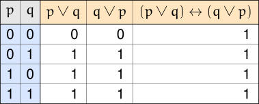
Example 1.5.6: Comparing $p \lor q$ and $q \lor p$
We may suspect that the order we list the atomic propositions in a
disjunction may not actually matter, but we can easily verify this with a
truth table:
So we now see that whenever we see a disjunction between two
propositions, we can swap the order without affecting the truth value.
Let’s see one more example of some “equivalent” expressions.
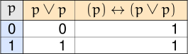
Example 1.5.7: Comparing $(p \lor p)$ and $(p)$
Again, let’s organize our results into a truth table:
Based on this example, we now know that if we ever see a proposition
disjunctioned with itself, we can just replace the entire disjunction
with a single copy of the atomic proposition used.
We just saw three examples of biconditionals that were tautologies. A
reasonable next question would be “so what?”
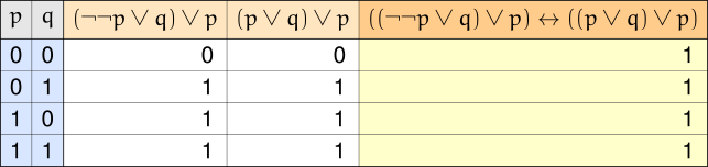
Example 1.5.8: Examining the proposition $(\neg \neg p \lor q) \lor p$
This proposition uses the three kinds of propositions we saw in the three
previous examples. We can probably guess where this example is leading,
but let’s continue on.
We’ve kept parentheses around every grouping here on purpose. We haven’t
justified anything about rearranging parentheses yet — only swapping the
order of a disjunction’s two sides, and collapsing a disjunction with
itself — so we’ll stick to those two moves and keep checking our work
with a truth table at every step.
We suspect we can replace $\neg \neg p$ with just $p$, like so, without
affecting the overall truth value:
So we can still replace $\neg \neg p$ with just $p$ and still get the
same truth values:
Previously we also saw that in a disjunction, we could swap the
propositions without affecting the overall truth value. Let’s see if we
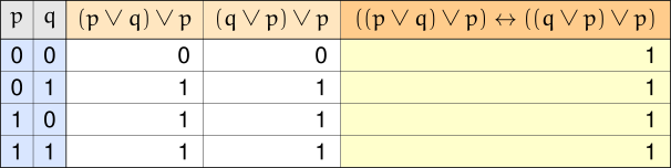
can swap out $p \lor q$ for $q \lor p$ without affecting the truth value:
Ok, we still get the same truth values under the same combinations of
truth values for $p$ and $q$.
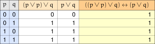
Let’s keep rearranging things this way, still checking our work with a
truth table at every step, until the two copies of $p$ end up sitting
right next to each other:
We also saw that we could replace a disjunction between a proposition and
itself with just that proposition. Since $(p \lor p)$ behaves just like
$p$, this leaves us with $p \lor q$ — matching what the table above
already confirms.
Hence we see that
Meaning the proposition $((\neg \neg p \lor q) \lor p) \leftrightarrow (p \lor q)$
is a tautology. Both $(\neg \neg p \lor q) \lor p$ and $(p \lor q)$ have
the exact same behavior under all combinations of truth values for $p$
and $q$.
In essence, what this means is that whenever we encounter the expression
$(\neg \neg p \lor q) \lor p$, we can fully understand it by examining
$(p \lor q)$ instead — we can basically just replace
$(\neg \neg p \lor q) \lor p$ with $(p \lor q)$ without affecting
anything.
Being as $(p \lor q)$ is much simpler than $(\neg \neg p \lor q) \lor p$ —
without all the extra copies of the $\neg$ symbol, the extra $\lor$
symbols, or the extra copy of proposition $p$ — we’d rather work with the
expression $(p \lor q)$.
The past couple of examples have demonstrated how complicated expressions
can be replaced (and better understood) with simpler expressions.
Logical Equivalence
The reason why we can replace a complicated proposition with a simpler
proposition is because that simpler proposition exhibits the exact same
behavior as the more complicated proposition when the atomic propositions
assume — or take — the same combination of truth values. By “the same
behavior,” we mean they have the same truth values, meaning the
biconditional is a tautology.
LOGICALLY EQUIVALENT
Two propositions $S_1$ and $S_2$ are called logically
equivalent, and we write
$$S_1 \Longleftrightarrow S_2$$
whenever the biconditional
$$S_1 \leftrightarrow S_2$$
is a tautology.
At least one of $S_1$ and $S_2$ needs to be compound for this to be
interesting. We actually already saw an example where only one side was:
$\neg \neg p$ is logically equivalent to just $p$, even though $p$ itself
is primitive. Comparing two primitive propositions to each other isn’t
nearly as useful — a primitive proposition’s truth value doesn’t depend
on the truth value of any other proposition, so there’s no combination of
truth values to check across.
Logical equivalence is the basis for the Laws of Logic.
Laws of Logic
The Laws of Logic are nothing more than a list of logical equivalencies.
Here, we present a rather long list of known logical laws.
$\begin{array}{c} p \land p \Longleftrightarrow p \\ p \lor p \Longleftrightarrow p \end{array}$
Identity Laws
$\begin{array}{c} p \land T_0 \Longleftrightarrow p \\ p \lor F_0 \Longleftrightarrow p \end{array}$
Inverse Laws
$\begin{array}{c} p \land \neg p \Longleftrightarrow F_0 \\ p \lor \neg p \Longleftrightarrow T_0 \end{array}$
Domination Laws
$\begin{array}{c} p \land F_0 \Longleftrightarrow F_0 \\ p \lor T_0 \Longleftrightarrow T_0 \end{array}$
Absorption Laws
$\begin{array}{c} p \land (p \lor q) \Longleftrightarrow p \\ p \lor (p \land q) \Longleftrightarrow p \end{array}$
Just like we did in the examples, all of the above can be verified by
examining a truth table containing a biconditional and determining
whether or not the biconditional is a tautology.
Some More Laws of Logic
There are a couple more logical equivalencies that prove to be useful.
In the previous section we saw an example where we used tautologically
true biconditionals to “simplify” complicated propositional expressions
into simpler propositional expressions. Whatever we could say about the
simpler expressions could also be said about their more complicated,
logically equivalent counterparts (except perhaps our preference for
working with the simpler expressions, of course).
In this section we do more work with logical equivalencies, similar to
what we saw in the examples seen previously. Our work here will bear a
striking resemblance to our experience in dealing with the arithmetic and
algebra of real numbers. In fact, the upcoming work we are about to
engage with has been dubbed the “algebra of propositions.”
Revisiting a Previous Example
In the previous example, we saw how to take a complicated proposition
and produce a simpler proposition that always had the same truth value.
Now that we have a big list of logical equivalencies under our belt, we
can see how to use those equivalencies to more quickly find equivalent
propositions, rather than trudge through truth tables all the time.
Example 1.6.1: Reexamining $(\neg \neg p \lor q) \lor p$
Previously, we made guesses about how the following propositions were
related to each other:
\[
\begin{align*}
& \neg \neg p \text{ compared to } p \\
& p \lor q \text{ compared to } q \lor p \\
& p \lor p \text{ compared to } p
\end{align*}
\]
and used what we found to make a bunch of truth tables, which is
reviewed below:
\[
\begin{align*}
\neg \neg p &\Longleftrightarrow p \\
p \lor q &\Longleftrightarrow q \lor p \\
p \lor p &\Longleftrightarrow p
\end{align*}
\]
Instead of using truth tables, let’s just use the laws of logic.
\[
\begin{array}{ll}
(\neg \neg p \lor q) \lor p \Longleftrightarrow (p \lor q) \lor p & \text{by the Law of Double Negation} \\
(p \lor q) \lor p \Longleftrightarrow (q \lor p) \lor p & \text{by the Commutative Law of } \lor \\
(q \lor p) \lor p \Longleftrightarrow q \lor (p \lor p) & \text{by the Associative Law of } \lor \\
q \lor (p \lor p) \Longleftrightarrow q \lor p & \text{by the Idempotent Law of } \lor \\
q \lor p \Longleftrightarrow p \lor q & \text{by the Commutative Law of } \lor
\end{array}
\]
We probably could have used fewer steps by more carefully applying the
commutative and associative laws, but regardless, we arrived at the same
proposition as we did in Example 1.5.4.
A New Example
Let’s turn our sights to a new example we haven’t seen before, and
compare using truth tables to using logical equivalencies.
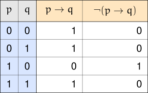
Example 1.6.2: $\neg (p \to q)$ via truth tables
We’re interested in seeing if there’s a simpler, equivalent way of
writing an expression like $\neg (p \to q)$ — one that doesn’t use the
implication, but is instead just a combination of conjunctions,
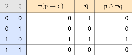
disjunctions, and negations. First, let’s construct a truth table for $\lnot (p \rightarrow q)$:
Suppose we didn’t know about the Laws of Logic. How can we proceed? We
notice that there is only one $1$ in the column for $\neg (p \to q)$. We
may remember that the conjunction of $p$ and $q$ also only has one $1$
as well.
However, the $1$s aren’t in the same row. Notice that if we swap the
$1$s and $0$s in the $q$ column, we can get the $1$s to line up with
those for $p$. But how do we swap $1$s and $0$s of a proposition?
We negate it! Let’s add $\neg q$ to the table.
Now we see that $\neg (p \to q)$ and $p \land \neg q$ have the same
truth values for all combinations of truth values, meaning
Using the truth table method required us to make keen observations on
how to work, manipulate, and coax truth values into the proper rows so
they line up.
What if we don’t see a way to make values line up? Fortunately, there is
a way we can avoid relying on our ability to make clever observations:
we use the Laws of Logic!
Example 1.6.3: $\neg (p \to q)$ via logical laws
Let’s use the Laws of Logic we have seen to try and come up with a
logically equivalent proposition:
\[
\begin{array}{lll}
& \boldsymbol{\neg (p \to q)} & \textbf{Reason} \\
\Longleftrightarrow & \neg (\neg p \lor q) & \text{Law of Material Implication} \\
\Longleftrightarrow & \neg \neg p \land \neg q & \text{DeMorgan's Law} \\
\Longleftrightarrow & p \land \neg q & \text{Law of Double Negation}
\end{array}
\]
This is the same proposition we got by using truth tables! We just used
logical equivalencies we were familiar with, instead of a keen eye
(which may have blind spots). There was also a lot less work involved
too!
A Note on Organizing Logical Equivalencies
In the previous example, we listed the logical equivalencies on
separate lines, citing the logical law being appealed to. This is
certainly a fine way to organize one’s work, and has its advantages.
In this book, we opt to use a tabular format to organize our work,
unless the occasion calls for some other format. We adopt a
three-column format:
One thing to notice is that initially, we had four atomic propositions:
$p$, $q$, $r$, and $s$. After all of our work above, we ended up with
only two: $p$ and $r$. This means that the large, complicated compound
proposition’s truth value actually is unaffected by $q$ or $s$. The
truth value is driven, or affected, only by $p$ and $r$.
Application: Switching Networks
While the content we’ve seen so far seems ethereal, with little application
outside of simplifying logical propositions, logic dictates almost every
avenue of study. In our everyday lives, we like to think our actions are
reasonable and make sense. Certainly, we can use logic to analyze a
situation so we can maximize our profit from it, whether our profit is in
the form of friendship, promotions at work, happiness, health, or money.
One such application of logic has had a profound impact on human history.
In 1938, a paper “A Symbolic Analysis of Relay and Switching Circuits” was
published. In that paper, author Claude Shannon showed that Boolean Logic
(what we’ve been studying so far in this book) can be used to simplify the
design of relay circuits that were used in the construction of
electromechanical devices back in the day. (Likewise, these relay circuits
could be used to solve Boolean algebra problems, essentially meaning that
relay circuits are equivalent to Boolean/propositional expressions.)
This insight paved the way for future computer advancements, culminating
in the development of modern computer chip designs, including modern CPU,
GPU, and now TPU chip designs.
In this section, we take a look at a very basic framework for taking
“complicated” circuits and producing equivalent, simpler circuits.
Electrical Circuits
An electrical circuit at its core is simply a network of switches that are
designed to allow or block electricity from flowing from one terminal to
another.
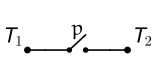
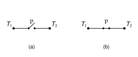
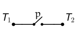
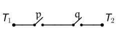
Here is the simplest switching network:
Here, $T_1$ is the starting terminal, and $T_2$ is the ending terminal.
Electrical current is applied at $T_1$.
Here, there is one switch, labeled $p$. In the diagram above, $p$ is
“open,” meaning it isn’t allowing electricity to flow through.
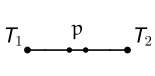
Here is the same circuit, with switch $p$ “closed,” thus allowing
electricity to flow:
The connection between these circuits and logic is this: open switches
correspond to false propositions, and closed switches correspond to true
propositions.
So, the first circuit we saw corresponds to when $p$ represents a false
proposition ($p = 0$). The second circuit corresponds to when $p$
represents a true proposition ($p = 1$).
Two Fundamental Circuits
Here we start by showing two circuits that are used to construct more
elaborate circuits.
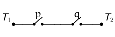
Here is the first:
In order for electricity to flow from terminal $T_1$ to terminal $T_2$,
both switches $p$ and $q$ must be closed ($p = 1$ and $q = 1$).
This is exactly the same as saying $p \land q$: when either $p$ or $q$ is
open (equal to $0$), then there isn’t a connected path from $T_1$ to
$T_2$. When both are closed (equal to $1$), then there is a path from
$T_1$ to $T_2$.
This circuit is called the “Series Circuit” and corresponds to the
conjunction operator.
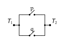
Here is the second fundamental type of circuit: the “Parallel Circuit”
Here, we see that as long as at least one of $p$ or $q$ is closed (at
least one of $p$ or $q$ is equal to $1$), then electricity can flow from
$T_1$ to $T_2$.
Of course, saying $p$ or $q$ must be closed is equivalent to the
disjunction of $p$ and $q$: when $p \lor q = 0$, electricity can’t flow
from $T_1$ to $T_2$. When $p \lor q = 1$, electricity can flow.
From just these two circuits, we can build up many useful circuits.
A Simple Example
The ability to simplify circuits relies on our ability to model a given
circuit as a proposition containing a combination of atomic propositions,
negations, conjunctions, and disjunctions.
We do that by identifying the series and parallel circuits being used in
the given circuit.
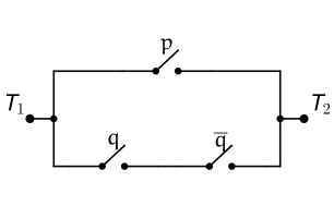
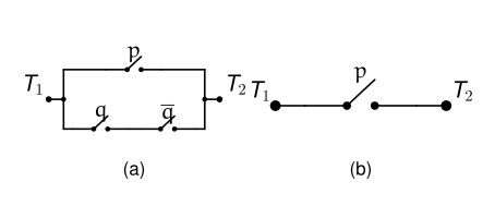
Example 1.7.1: Our First Example
This is a parallel circuit between a single switch $p$ and a series
circuit consisting of $q$ and $\neg q$.
Thus, we model this circuit as
$$p \lor (q \land \neg q)$$
Now, we can use the laws of logic to simplify this proposition:
\[
\begin{array}{lll}
& \boldsymbol{p \lor (q \land \neg q)} & \textbf{Reason} \\
\Longleftrightarrow & p \lor F_0 & \text{Inverse Law of } \land \\
\Longleftrightarrow & p & \text{Identity Law}
\end{array}
\]
So, we can simplify $[p \lor (q \land \neg q)]$ to just $p$. The circuit
for $p$ is below:
We have just produced a circuit that is equivalent to the circuit we were
given, but is much simpler:
A Complex Example
We can take a more complicated circuit and do the same thing:
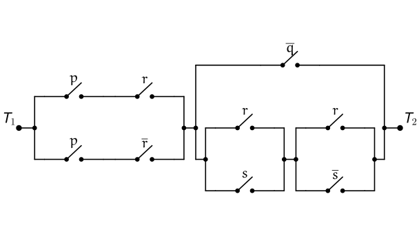
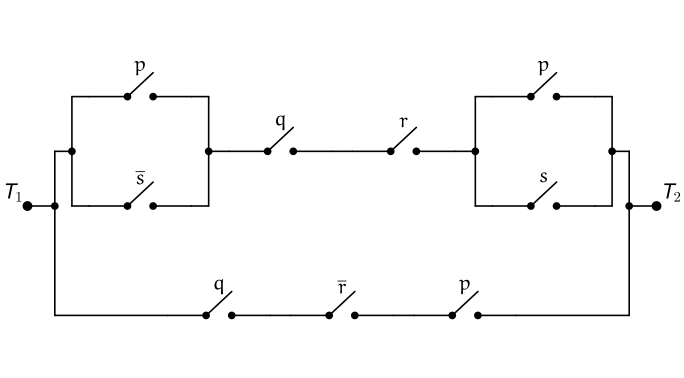
Example 1.7.2: A More Complicated Example
Consider the following circuit:
There are two sub-circuits connected in series:
$$[\quad] \land [\quad]$$
The first part is a parallel circuit consisting of a series circuit along
each branch:
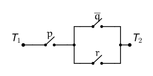
This final proposition doesn’t seem to admit any further simplifications
using the laws of logic at our disposal.
As such, we accept this final proposition for our simplified circuit:
Obfuscating Circuits
Something we could do, if we were worried someone may take our circuit
designs, is to obfuscate them by taking a simple circuit and using the
laws of logic “in reverse,” so to speak, to produce an equivalent, more
complicated circuit.
Example 1.7.3: Designing a Complicated Plumbing Network
A deranged mad man is planning to abduct a group of people and force them
to solve a series of puzzles to survive.
One such puzzle involves opening and closing a network of valves designed
to carry a liquid antidote to a poison the mad man will administer to his
victims. If the kidnapped individuals can configure the valves in a
satisfiable way, the liquid antidote will be carried through the plumbing
network to vials the victims can drink from.
Initially, the mad man starts with just
$$p \land q$$
but wants to design a more complicated network to hide the simplicity, so
the lunatic uses the laws of logic in the following way:
So essentially, we started with the following plumbing circuit:
and constructed the following circuit:
The mad man is pleased with his new design, and implements it for his
plan. Or he would have, had he not been caught by investigators for his
recent tax fraud schemes.
In the previous example, we saw how the laws of logic can be used to turn
simple propositions into more complex ones. For example, a combination of
the identity laws and inverse laws allow us to introduce superfluous
atomic propositions.
We also saw that propositions can be used to model non-electric networks
as well, such as a valved plumbing network. Any kind of gated network can
be modeled as a proposition.
Open Propositions
All of the propositions we’ve dealt with so far have had definite truth
values. For example,
$$\text{Thomas Jefferson was the second president of the United States.}$$
is a proposition that is known to be false. A statement such as
$$\text{2 + 2 = 4, or 2 + 2 = 5.}$$
is a compound proposition that is true.
However, a statement such as
$$\text{$n$ is 1 more than a multiple of 3.}$$
is not a proposition, because we don’t know whether it’s true or false. We
would need to know the value of $n$ in order to reach such a conclusion.
For example, the statement is false when $n = 5$, but true when $n = 16$.
Here, we’ll deal with sentences involving variables like this one.
Open Statements
Example 1.8.1: A statement whose truth value depends on a variable
Consider the statement
$$x + 3 = 8.$$
Here, we aren’t asking what value of $x$ solves the equation (we could,
but that isn’t our focus). Instead, we’re asking whether, given a
specific value of $x$, the statement is a true proposition or a false
proposition.
We start by modeling the statement using a letter, like we’ve done up to
this point, but we also use parentheses to denote the variable $x$:
Both of these examples are open statements — sentences with variables
whose truth value can’t be pinned down until we substitute something in
for those variables.
OPEN STATEMENT
An open statement is any declarative sentence that has one or more
variables, and thus is not a proposition, but becomes a proposition after
values are substituted for all of its variables.
Just like with ordinary propositions, we write $p(x) = 0$ if the value of
$x$ makes $p(x)$ a false proposition, and $p(x) = 1$ if the value of $x$
makes $p(x)$ a true proposition.
PROPOSITIONAL FUNCTION
A statement $p(x)$ that represents an open statement with variable $x$ is
often called a propositional function.
A propositional function can depend on more than one variable, as the
next example demonstrates.
Example 1.8.3: A propositional function with three variables
The U.S. Postal Service will only ship a package in a box that meets
certain requirements: the sum of the box’s length and girth must not
exceed 108 inches, where the girth is the perimeter of the box’s
rectangular cross section.
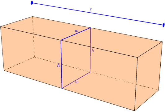
Letting $\ell$, $w$, and $h$ represent a
box’s length, width, and height respectively, the perimeter of that
cross section is $2w + 2h$. So, to comply with USPS shipping
requirements, we need
$$\ell + 2w + 2h \leq 108 \text{ inches.}$$
We can model this situation using a propositional function with three
variables:
Since $116 \not\leq 108$, we can’t ship a box with length $20$ inches,
width $18$ inches, and height $30$ inches with USPS.
Constraining Inputs
Let’s reconsider the president example.
Example 1.8.4: Restricting inputs to remove ambiguity
For the propositional function
\[
\begin{array}{rl}
p(x)\text{: } &x \text{ was the 30th president of the United States,}
\end{array}
\]
we could argue $p(3)$ is either false or undefined. We can
eliminate this ambiguity by specifying what kinds of values we’re
allowed to substitute into $p(x)$. If a value $a$ is allowed as an input,
then $p(a)$ is either true or false. If a value $b$ is not allowed, then
$p(b)$ is undefined.
Let’s restrict the values allowed as inputs to $p(x)$ to proper names.
This means values like “James K. Polk,” “Cecil Rhodes,” “Grover
Cleveland,” “Calvin Coolidge,” and “Bill Clinton” can be substituted for
$x$ and will yield true or false.
However, when substituting a value for $x$ that isn’t a proper name,
we’ll say $p(x)$ is undefined. Since $3$ isn’t a proper name, $p(3)$ is
undefined.
We could further restrict the inputs to be names of U.S. presidents
only, rather than just any proper name. In that case, $p(\text{Cecil
Rhodes})$ would be undefined, since “Cecil Rhodes” isn’t the name of any
U.S. president.
Example 1.8.5: Restricting inputs can force every output to agree
Reconsider the propositional function
\[
\begin{array}{rl}
p(x)\text{: } &x \text{ was the 30th president of the United States.}
\end{array}
\]
Suppose we restrict the allowable values to names of U.S. presidents,
except “Calvin Coolidge.” Then $p(\text{Calvin Coolidge})$ would be
undefined. Substituting any other U.S. president’s name yields $0$,
since only Calvin Coolidge was the 30th U.S. president. Under this
restriction, $p(x)$ never yields $1$ — only $0$, or undefined.
Restricting the allowable names to Spanish monarchs would also only ever
yield $0$ or undefined, since no Spanish monarch was ever the 30th
president of the United States. We could similarly restrict the
allowable values to even integers — again, $p(x)$ would always be either
false, or undefined.
Example 1.8.6: The same restriction can change which values are undefined
If we restrict our inputs to integers only, we can make $p(x)$ true by
substituting $5$ in for $x$. Any other integer yields $0$. Non-integers
yield undefined values, since they aren’t allowed as inputs — so
$p(3.14159265)$ is undefined.
However, if we restrict allowed inputs to any real number, $p(3.14159265)$
is no longer undefined — it’s equal to $0$.
The previous examples show that restricting the allowable inputs of a
propositional function can greatly affect the truth values it yields.
This collection of allowable values has a special name, and knowing what
it consists of is vitally important.
UNIVERSE OF DISCOURSE, UNIVERSE
For a given propositional function $p(x)$, the collection of values
allowed to be substituted in for $x$ is called the universe of
discourse, or just universe for short.
The universe is typically denoted $\mathcal{U}$, though other symbols
may be used.
Example 1.8.7: Checking whether a value belongs to the universe
Consider the propositional function
\[
\begin{array}{rl}
r(x)\text{: } &x \text{ has a right angle,}
\end{array}
\]
with universe of discourse $\mathcal{U}$ the collection of all planar
polygons.
Since the number $2$ isn’t a planar polygon, $r(2)$ is undefined.
Suppose $s_1$ represents a square with side length $1$. $s_1$ is a
planar polygon, meaning $r(s_1)$ is either $0$
or $1$. Since every square has a right angle, $r(s_1) = 1$.
Suppose $s_2$ represents an equilateral triangle with side length $1$.
$s_2$ is also a planar polygon. Since no
equilateral triangle has a right angle, $r(s_2) = 0$.
As demonstrated earlier, a propositional function can have many
variables — we’d need to specify the universe of discourse that all of
those variables have to adhere to.
Example 1.8.8: One shared universe for every variable
Consider the propositional function
\[
\begin{array}{rl}
e(x, y)\text{: } &x + y \text{ is an even integer,}
\end{array}
\]
with universe of discourse $\mathcal{U}$ for both $x$ and $y$ the
integers. This means both $x$ and $y$ must be integers.
We’d have $e(2, 4) = 1$, $e(3, 7) = 1$, $e(1, 2) = 0$, and $e(4, 13) = 0$.
$e(2, 2.3)$, $e(2.18, 3.14)$, and $e(4.411, 10)$ would all be undefined,
since $2.3$, $2.18$, $3.14$, and $4.411$ aren’t integers.
$e(2, \text{Monday})$ would also be undefined, since “Monday” isn’t an
integer. Similarly, $e(\text{Red}, \text{Cactus})$ would also be
undefined.
For $e(x, y)$ to yield $0$ or $1$, both $x$ and $y$ need to be integers.
It’s also possible to specify a separate universe for every variable in
a propositional function.
Example 1.8.9: A separate universe for each variable
Consider the propositional function
\[
\begin{array}{rl}
q(x, y)\text{: } &x \div y \text{ is larger than 5.2,}
\end{array}
\]
with universe for $x$, denoted $\mathcal{U}_x$, all real numbers, and
universe for $y$, denoted $\mathcal{U}_y$, all real numbers except $0$.
$q(1, 0)$ would be undefined, since $0 \notin \mathcal{U}_y$.
$q(\text{Monday}, 1)$ would be undefined, since $\text{Monday}$ is not a real number.
$q(\text{Friday}, 0)$ would be undefined, since $\text{Friday}$ is not a real number, and $0$
is not a non-zero real number.
Of course, it’s also possible for some of a propositional function’s
variables to share a universe of discourse, while others have some other
universe.
Example 1.8.10: Some variables sharing a universe, others not
Consider the propositional function
\[
\begin{array}{rl}
q(x, y, z)\text{: } &(x + y) \div z = 1,
\end{array}
\]
with universe for $x$ and $y$, denoted $M$, all integers, and universe
for $z$, denoted $N$, all real numbers except $0$.
We have $q(1, 0, 1) = 1$, $q(-2, 7, 5) = 1$, $q(-1, 1, 1) = 0$, and
$q(10, -23, 2) = 0$.
$q(0.1, 1, 1)$ is undefined, since the supplied value for $x$ ($0.1$)
isn’t in $M$.
Similarly, $q(23, -3.14, 10)$ is undefined, since the supplied value for
$y$ ($-3.14$) isn’t in $y$’s universe, $M$.
Finally, $q(20, -10, 0)$ is undefined, since the supplied value for $z$
($0$) isn’t in $z$’s universe, $N$.
Quantifiers
Consider the following propositional functions, both defined on the
universe $\mathcal{U}$ of all integers:
\[
\begin{array}{rl}
s(n)\text{: } &n^2 \text{ is even.} \\
t(m, n)\text{: } &m^2 - n^2 \text{ is even.}
\end{array}
\]
We can find values of $n$ that make $s(n)$ true, such as $n = -4$. We can
also find values of $n$ that make $s(n)$ false, such as $n = 13$. The
same is true of $t(m, n)$: the values $m = 3$ and $n = -7$ make $t(m, n)$
true, while $m = 4$ and $n = -1$ make $t(m, n)$ false.
Now consider the following statements:
\[
\begin{array}{rl}
\alpha\text{: } &\text{For some } n \text{, } s(n) \text{ is true.} \\
\beta\text{: } &\text{For all } m \text{ and all } n \text{, } t(m, n) \text{ is true.}
\end{array}
\]
$\alpha$ and $\beta$ aren’t open statements, even though variables show
up in them. The difference is that each statement is making a specific
claim, and the truth value of that claim doesn’t depend on the values
taken by the variables.
Statement $\alpha$ is claiming that some specific integer exists that
makes $s(n)$ true. As we saw above, one such value is $n = -4$, so
$\alpha$ is a true proposition. It doesn’t matter that $n = 13$ makes
$s(n)$ false — $\alpha$ is only claiming that some satisfying value
exists, and we already found one.
Likewise, $\beta$ is making a specific claim: that every single value
of $m$ and every single value of $n$ makes $t(m, n)$ true. We saw that
$t(m, n)$ is false when $m = 4$ and $n = -1$. Because it isn’t true that
every $m$ and every $n$ make $t(m, n)$ true, $\beta$ is a false
statement — regardless of the fact that some values of $m$ and $n$ do
make $t(m, n)$ true.
We explore these kinds of statements here, and in the next couple of
sections.
The Existential Quantifier
The phrases “for some $n$” (used in statement $\alpha$) and “for all $m$
and all $n$” (used in statement $\beta$) are said to quantify the
propositional functions $s(n)$ and $t(m, n)$.
The following phrases are all equivalent, and specify the existential
quantifier:
“for some $x$”
“for at least one value of $x$”
“a value of $x$ exists such that”
“an $x$ exists such that”
EXISTENTIAL QUANTIFIER
The phrase “for some $x$,” specifying that at least one value of $x$
exists that satisfies some condition, is called the existential
quantifier.
The existential quantifier can be expressed symbolically as $\exists x$.
For any propositional function $p(n)$, we can consider the statement
$$\exists n\ p(n)$$
which is equivalent to the statement “For some $n$, $p(n)$,” which in
turn is equivalent to saying “For some $n$, $p(n)$ is true.” Note that in
the first two phrasings, we omit the “is true” part — it’s assumed that
we’re considering the existence of values of $n$ that make $p(n)$ true.
We could also consider the existence of values of $n$ that make $p(n)$
false, by considering the statement
$$\exists n\ \neg p(n).$$
Similarly, we can use logical connectives along with the existential
quantifier. So for propositional functions $x(n)$ and $y(n)$, we can
consider the statements
where we enclose the propositional functions in brackets to specify that
the existential quantifier applies to the whole logical connective. This
is different from the statements
where the existential quantifier only applies to the propositional
function $x(n)$. In general, it’s a good idea to enclose whatever
statement you want a quantifier applied to in brackets.
At this point, it’s worth pointing out that $p(x)$ is an open statement,
whose truth value can only be determined after substituting in a value
for $x$ from some universe of discourse, whereas $\exists n\ p(n)$ is not
an open statement — it has a definite truth value (either some value of
$x$ from the universe exists such that $p(x) = 1$, or no such value
exists).
It’s also worth pointing out that when we say something like
$\exists n\ p(n) = 1$, we mean that the statement $\exists n\ p(n)$ is
equal to $1$ — we are not simply saying that $p(n) = 1$ (again, because
$p(n)$ is an open statement, we’d have to substitute a value in for $n$
before we know whether $p(n) = 0$ or $p(n) = 1$).
Remember that, by definition, a statement such as $\exists n\ p(n)$ is
true if we can find at least one value of $n$ that makes $p(n) = 1$.
There could be infinitely many such values, $1000$ values, $10$ values,
or even exactly $1$ value — the existence of at least one such value is
enough to make $\exists n\ p(n)$ a true statement.
Example 1.9.1: Existentially quantified statements
Consider the universe of all real numbers, along with the following open
statements:
The statement $\exists x\ [p(x) \land r(x)]$ is true, because there
exists at least one value of $x$ ($x = 1$) that makes both $p(x) = 1$ and
$r(x) = 1$. We can translate this statement as “There exists a value of
$x$ such that $x \geq 0$ and $1 - x^2 = 0$.”
The statement $\exists x\ [p(x) \to q(x)]$ is true, because
there exists at least one value of $x$ ($x = -1$) such that $p(x) = 0$,
$q(x) = 1$, and $0 \to 1$ is true. Another value that makes
this statement true is $x = 5$, since $p(5) = 1$, $q(5) = 1$, and
$1 \to 1$ is true. We can translate this statement as “There
exists at least one value of $x$ such that if $x \geq 0$, then
$x^2 \geq 0$.”
The statement $\exists x\ [r(x) \lor s(x)]$ is true, because there exists
a value of $x$ (such as $x = 4$) where $r(x) \lor s(x) = 1$, since
$r(4) = 0$ and $s(4) = 1$. We can translate this statement as “There
exists a value of $x$ such that $1 - x^2 = 0$, or $x^2 - 3x + 2 > 0$.”
Showing that an existentially quantified statement is false is harder
than showing one is true, because it isn’t enough to come up with a
single example — it must be demonstrated that every single value
within the universe of discourse yields a false statement. To be clear,
for an open statement such as $p(x)$, what we’re talking about is
showing that $\neg \exists x\ p(x)$ is true by showing that
$\exists x\ p(x)$ is false. This is different from asking about the
truth value of $\exists x\ [\neg p(x)]$.
Example 1.9.2: Showing an existentially quantified statement is false
For the universe of discourse of all natural numbers (integers larger
than $0$, not including $0$), consider the following open propositions:
\[
\begin{array}{rl}
a(n)\text{: } &n^2 + 1 = 1 \\
b(n)\text{: } &2n + 1 \text{ is an even number.} \\
c(n)\text{: } &n^2 + 2 \text{ is a perfect square.}
\end{array}
\]
The statement $\exists n\ [a(n)]$ is false, because the only integer
where $n^2 + 1 = 1$ is $n = 0$ — but $0$ isn’t in our universe of
discourse, meaning $a(0)$ is undefined. As such, $\exists n\ [a(n)]$ is
false, and $\neg \exists n\ [a(n)]$ is true.
The statement $\exists n\ [b(n)]$ is false, because $1$ more than any
multiple of $2$ is, by definition, odd — so no integer exists such that
doubling it and adding $1$ results in an even integer. Hence,
$\neg \exists n\ [b(n)]$ is true.
The statement $\exists n\ [c(n)]$ is false. Consider the difference
between $n^2$ and $(n+1)^2 = n^2 + 2n + 1$. For any integer greater than
$0$, the value $2n + 1$ is larger than $2$, so it isn’t possible to form
a perfect square by adding $2$ to a previous perfect square. Hence,
$\neg \exists n\ [c(n)]$ is true.
The Universal Quantifier
The following phrases are all equivalent, and specify the universal
quantifier:
“for all $x$”
“for any $x$”
“for each $x$”
“for every $x$”
UNIVERSAL QUANTIFIER
The phrase “for all $x$,” specifying that every value of $x$ satisfies
some condition, is called the universal quantifier.
The universal quantifier can be expressed symbolically as $\forall x$.
The statement $\forall x\ p(x)$ asserts that all values of $x$ make
$p(x)$ true. The statement $\forall x\ \neg p(x)$ asserts that all
values of $x$ make $p(x)$ false. Again, it’s advisable to use brackets to
specify how the quantifier is being used, as in $\forall x\ [p(x)]$ and
$\forall x\ [\neg p(x)]$.
Example 1.9.3: Universally quantified statements
Consider the universe of all real numbers, along with the following open
statements:
The statement $\forall x\ [q(x)]$ is true, because no matter what real
number we square, the result is always greater than or equal to $0$.
As such, the statement $\forall x\ [p(x) \to q(x)]$ is also
true, because squaring a positive number always yields a positive
number.
The statement $\forall x\ [p(x) \land s(x)]$ is false, because
$p(1.5) \land s(1.5) = 1 \land 0 = 0$. Thus, $x = 1.5$ is a
counter-example.
The statement $\forall x\ [\neg p(x) \lor r(x)]$ is false, because
$\neg p(0) \lor r(0) = \neg(1) \lor 0 = 0 \lor 0 = 0$. As such, $x = 0$
is a counter-example, proving $\forall x\ [\neg p(x) \lor r(x)]$ is
false.
Explicit and Implicit Quantification
Some open propositions may not be as explicitly stated as we’d like.
Determining whether a statement uses an existential or universal
quantifier may require a close look at its wording, or some outside
knowledge.
Example 1.9.4: An implicitly universally quantified statement
Consider a universe $A$ consisting of all animal species (sponges, ants,
kangaroos, elephants, etc.), along with the two following sentences:
If an animal flies, then it has wings.
If $x$ is a flying animal, then $x$ has wings.
Both sentences express the same idea, but are they open statements? The
second sentence does have a variable, but neither sentence uses a
construct like “All $x$,” “For all $x$,” “Every $x$,” “Some $x$,” or
even “An $x$ exists such that…”
The presence of the indefinite articles “a” and “an” suggests that both
statements use the universal quantifier, since they’re imposing a
condition, and every animal in the universe can be checked against it.
So, the universal quantifier is being used implicitly here, not
explicitly.
Let’s introduce the propositional functions
\[
\begin{array}{rl}
f(x)\text{: } &x \text{ is a flying animal.} \\
w(x)\text{: } &x \text{ is an animal with wings.}
\end{array}
\]
We can rewrite both bulleted statements above in a more mathematically
precise way, using the universal quantifier, as
$$\forall x\ [f(x) \to w(x)].$$
Example 1.9.5: A second implicitly universally quantified statement
Consider a universe $Q$ consisting of all planar quadrilaterals, along
with the following sentence:
$$\text{The opposite angles of a cyclic quadrilateral are supplementary, and conversely.}$$
Again, this sentence lacks any of the usual linguistic constructs that
explicitly determine which quantifier is used. The only clue that the
universal quantifier is used is the indefinite article “a.”
Using the propositional functions
\[
\begin{array}{rl}
c(q)\text{: } &q \text{ is a cyclic quadrilateral.} \\
s(q)\text{: } &\text{The opposite angles of } q \text{ are supplementary.}
\end{array}
\]
we can rewrite the sentence above in a mathematically precise way as
$$\forall q\ [c(q) \leftrightarrow s(q)].$$
(The word “conversely” tells us that the converse of the statement is
also true. We could rewrite the sentence above as “If the opposite
angles of a quadrilateral are supplementary, then that quadrilateral is
cyclic, and conversely,” or as “The opposite angles of a quadrilateral
are supplementary if and only if the quadrilateral is cyclic.”)
Example 1.9.6: An implicitly existentially quantified statement
Consider the universe $I$ consisting of all the integers, along with the
statement
For this implicitly quantified statement, the word “has” suggests we’re
dealing with the existential quantifier. As such, we rewrite this
statement as
$$\exists x\ [x^3 - 6x^2 + 11x - 6 = 0].$$
A Quick Word on Notation
In every example so far, we’ve specified a universe of discourse, and
it’s been implicitly understood that all substitutions for variables
come from that universe. We can make this more explicit.
For example, up to now, we’d say something like “For some universe
$\mathcal{U}$, consider the statements $\forall x\ [p(x)]$ and
$\exists x\ [p(x)]$,” where we substitute values from the universe
$\mathcal{U}$ in for the variable $x$. We can instead write “Consider the
statements $\forall x \in \mathcal{U}\ [p(x)]$ and
$\exists x \in \mathcal{U}\ [p(x)]$,” using the symbol $\in$ (a stylized
Greek letter epsilon) to indicate that $x$ represents some value from the
collection $\mathcal{U}$. A construct such as “$x \in \mathcal{U}$” is
read as “$x$ is an element residing in universe $\mathcal{U}$.”
By extension, when we say something like “$\forall x \in \Psi\ [p(x)]$,”
we’re saying that for all values $x$ found within a universe, which we’re
denoting $\Psi$ (a capital Greek letter psi), $p(x)$ is a true statement.
Alternatively, when we write something like “$\exists x \in \Psi\
[p(x)]$,” this is equivalent to saying there exists some value, which
we’ll refer to as $x$, residing in a universe denoted by the Greek letter
$\Psi$, such that $p(x)$ is a true statement.
Quantified Laws of Logic
What can we deduce from knowing that a universally quantified open
statement is true? What can we deduce from knowing that an existentially
quantified statement is true? How are universally quantified statements
and existentially quantified statements related to each other? In this
section, we dig deeper into quantifiers, and explore propositional logic
involving them.
A Simple Definition
Just like with ordinary statements, we can ask whether two open
statements are logically equivalent.
LOGICALLY EQUIVALENT
Consider open statements $p(x)$ and $q(x)$ defined on some universe
$\mathcal{U}$.
When $p(a) \leftrightarrow q(a) = 1$ for every value $a$ within
$\mathcal{U}$ — in other words, when $p(a) \leftrightarrow q(a)$ is a
tautology — we say $p(x)$ and $q(x)$ are logically equivalent open
statements, and we write
$$\forall x\ [p(x) \Longleftrightarrow q(x)].$$
Example 1.10.1: Logically equivalent open statements
Consider the universe of all planar triangles, along with the open
statements
\[
\begin{array}{rl}
a(t)\text{: } &\text{All three angles of triangle } t \text{ are } 60°. \\
s(t)\text{: } &\text{All three sides of triangle } t \text{ have equal measure.}
\end{array}
\]
From classical geometry, we know that for any particular triangle
$\triangle ABC$,
For $q_1(x)$, we have $q_1(1) = 1$ and $q_1(2) = 1$; every other value of
$x$ yields $q_1(x) = 0$. For $q_2(x)$, we have $q_2(-1) = 1$ and
$q_2(-2) = 1$; every other value of $x$ yields $q_2(x) = 0$.
Since no value of $x$ makes $q_1(x) \land q_2(x)$ true, we have
It’s also worth pointing out that $\exists x\ [q_1(x)] \lor \exists x\
[q_2(x)] = 1$.
The previous example shows that the existential quantifier does not
distribute over the conjunction operator $\land$. In other words, for
general open statements $p(x)$ and $q(x)$,
It’s still true that whenever $\exists x\ [p(x) \land q(x)]$ holds,
$\exists x\ [p(x)] \land \exists x\ [q(x)]$ holds as well — it’s just the
reverse direction that can fail, as the previous example showed.
since if a value of $x$ within the universe exists that satisfies the
disjunction, one of the statements in the disjunction must be true. So,
the existential quantifier distributes over disjunction.
Example 1.10.3: The universal quantifier doesn’t distribute over disjunction
Consider the universe of all positive integers, along with the
propositional functions
For some open statement $p(x)$ and universe $\mathcal{U}$, what do
$\neg \exists x\ [p(x)]$ and $\neg \forall x\ [p(x)]$ mean, exactly?
Focus first on $\neg \exists x\ [p(x)]$. Remember that $\exists x\
[p(x)]$ asserts that at least one value of $x$ makes $p(x)$ true. If we
negate that statement, we’re saying that zero values of $x$ make
$p(x)$ true (it’s nonsensical to talk about a negative or fractional
number of satisfying values, so we can ignore those). Thus,
$\neg \exists x\ [p(x)]$ asserts that no value of $x$ makes $p(x)$ true —
in other words, every value of $x$ makes $p(x)$ false. This is
equivalent to $\forall x\ [\neg p(x)]$, so
Now consider $\neg \forall x\ [p(x)]$. Remember that $\forall x\ [p(x)]$
asserts that every value of $x$ makes $p(x)$ true. So, naturally, the
negation of $\forall x\ [p(x)]$ means that not every value of $x$ makes
$p(x)$ true — hence, there must exist at least one value of $x$ that
makes $p(x)$ false. This is equivalent to $\exists x\ [\neg p(x)]$, so
In an earlier section, we examined propositional functions with two and
three variables. For each variable in an open statement, we needed to
substitute some value from the respective universe in order to determine
the statement’s truth value.
Here, we look at quantifying statements with two or more variables.
Bound and Free Variables
BOUND VARIABLE, FREE VARIABLE
For some universe $\mathcal{U}$, consider a propositional function
$p(x, y)$ where $x$ and $y$ are both constrained by $\mathcal{U}$, and
the quantified statements
In both statements, $x$ is bound by a quantifier, while $y$ is not
bound by any quantifier. We say $x$ is a bound variable, while $y$ is a
free variable.
Up to now, we’ve only dealt with quantified statements with a single
variable — in every one of those examples, that variable was bound by
whatever quantifier was used, and every quantified statement had a
definite truth value.
In our definition above, any variable not bound by a quantifier is
called a free variable. As such, statements like $\forall x\ [p(x, y)]$
and $\exists x\ [p(x, y)]$ don’t have a definite truth value. In both
cases, we still need to either bind the variable $y$ with a quantifier,
or substitute a value in for it from $\mathcal{U}$, before the truth
value can be determined. This is important enough to highlight.
Quantified Statements with Free Variables Are Open Statements
For some universe $\mathcal{U}$, consider a propositional function
$p(x, y)$ where $x$ and $y$ are both constrained by $\mathcal{U}$, and
the quantified statements
The truth value of both statements is undetermined. As such, they are
open statements, whose truth values depend on what value is substituted
in for the free variable $y$.
Example 1.11.1: A quantified statement with a free variable
Consider the universe $N$ of all integers, along with the open statement
What happens when we quantify the $m$ variable? With the universal
quantifier, we get $\forall m\ [p(m, n)]$, which translates to “For every
integer $m$, we have that $m + n = 0$.” Is this true? We’d need to know
what value $n$ holds to be sure — we can’t just pick any value of $n$.
The statement would be false when $m = 1$ and $n = 2$. We just can’t be
sure, so $\forall m\ [p(m, n)]$ doesn’t have a definite truth value.
Now consider the statement $\exists m\ [p(m, n)]$, which translates to
“There exists an integer $m$ such that $m + n = 0$.” Again, until a
value for $n$ is known, we can’t be sure — though we could figure out
what value $n$ would need to be in order for $m + n = 0$ to hold. For
example, when $m = 5$, we could set $n = -5$. But the value of $n$ is
still unknown, so the statement $\exists m\ [p(m, n)]$ is open, and has
no definite truth value.
Repeated Quantifiers
In order for a quantified statement to have a definite truth value,
there can be no free variables. We can bind every variable with the same
kind of quantifier, which is useful, since there are many mathematical
statements we can make that rely on more than one variable.
Example 1.11.2: Order doesn’t matter when the same quantifier repeats
A basic law of arithmetic is the commutative law — in a sum or product,
the two constituent parts can be swapped without affecting the result.
In other words, for any two real numbers $x$ and $y$,
$$x + y = y + x.$$
Consider the universe $\mathcal{U}$ of all real numbers. We can express
the commutative laws of arithmetic using quantifiers like this:
$$\forall x\ \forall y\ [x + y = y + x] \qquad \forall x\ \forall y\ [x \cdot y = y \cdot x].$$
The order of the quantified variables doesn’t matter, so we could also
express the commutative laws of arithmetic like this:
$$\forall y\ \forall x\ [x + y = y + x] \qquad \forall y\ \forall x\ [x \cdot y = y \cdot x].$$
Example 1.11.3: Repeated existential quantifiers
Consider the universe $N$ consisting of all integers, along with the
statement
$$\text{The integer 100 is the sum of two perfect squares.}$$
The presence of the definite article “the” suggests that the existential
quantifier is implied here. As such, we could express the statement
using quantifiers like this:
$$\exists m\ \exists n\ [100 = m^2 + n^2].$$
Again, the order of quantification doesn’t matter in this case, so we
could also write $\exists n\ \exists m\ [100 = m^2 + n^2]$.
One more way to write this is to specify which universe each variable
belongs to using the $\in$ symbol:
$$\exists m \in N\ \exists n \in N\ [100 = m^2 + n^2].$$
Notice that when the same quantifier is used, the order in which we
express the quantification didn’t matter — this gives us our first
logical equivalency for repeated quantifiers.
Order Doesn’t Matter in Repeated Quantifiers
Consider a universe $\mathcal{U}$ for some open statement $p(x, y)$ with
variables $x$ and $y$:
This also applies to open statements involving three, four, or more
variables.
There’s a shorthand notation commonly used with repeated quantifiers.
For some universe $\mathcal{U}$ and the open statement $p(x, y)$, we can
use the following conventions:
Of course, this can be extended to as many variables as needed.
Example 1.11.4: Using the shorthand notation
Consider the universe of all real numbers, which we’ll denote $R$. When
dealing with real numbers, another commonly used arithmetic law is the
distribution of multiplication over addition, typically expressed as
“For every real number $x$, $y$, and $z$, $x(y + z) = xy + xz$.”
Here, the quantifier being used is the universal quantifier, applied to
every variable, so we can concisely represent this statement with the
proposition
Using the shorthand notation above, we could also write this as
$$\forall x, y, z\ [x(y + z) = xy + xz].$$
Mixed Quantifiers
Some statements involve both the existential quantifier and the
universal quantifier.
Example 1.11.5: Additive inverses, quantified
Consider the universe of all real numbers. It’s known that every number
has an additive inverse:
$$\text{For every real number } x \text{, there exists some other number } y \text{ where } x + y = 0.$$
Notice that we used the phrases “For every…” and “There exists…,” which
suggests both a universal quantifier and an existential quantifier. The
phrase “For every…” comes first, suggesting it’s the first quantifier,
with the existential quantifier coming second. As such, we can rewrite
the statement above as
$$\forall x\ \exists y\ [x + y = 0].$$
Since $x$ is universally quantified, we can pick arbitrary values to
test. If $x = 3008$, then $y = -3008$ will work. Similarly, taking
$x = -\pi^2$, we can set $y = \pi^2$. In fact, as soon as a value of $x$
is selected, we can just take $y = -x$, since $x$ being a real number
means $-x$ is too. So no matter what real number we pick for $x$, we can
always find an appropriate value for $y$.
Example 1.11.6: Swapping mixed quantifiers changes the meaning
Let’s reconsider the additive inverse example. Suppose we swapped
quantifiers, like we did when examining repeated quantifiers. Doing so
forms the statement
$$\exists y\ \forall x\ [x + y = 0].$$
This can be translated into English as “There exists some real number
$y$, such that for every real number $x$, we have $x + y = 0$.” Here,
the proposition asserts the existence of some such real number — and
supposedly, once it’s found, every real number added to it yields a sum
of $0$.
We know $y$ can’t be $17$, because $3 + 17 \neq 0$ (here, $y = 17$ and
$x = 3$). Similarly, $y$ can’t be $-0.745$, because $20 - 0.745 \neq 0$
(here, $y = -0.745$ and $x = 20$).
As a matter of fact, no such value of $y$ can exist. As soon as we pick
a value for $y$, there are infinitely many ways to pick the value of
$x$ — and since $x$ is universally quantified, the statement asserts that
every value of $x$ will work, which so far isn’t the case. Out of
those infinitely many sums, only one will be $0$: when $x$ is equal to
$-y$. Since $x$ is universally quantified, we could also pick the real
number $-y + 1$, which yields a sum of $1$, not $0$.
Surprisingly, if this statement were true, every single real number
would need to be equal to $0$ — an obviously ridiculous scenario!
Based on the two previous examples, we know that we can’t just swap
mixed quantifiers arbitrarily. Perhaps under very specific circumstances
it could be done, but in general, it isn’t something we can do. This is
worth highlighting.
Mixed Quantifiers are Generally Unswappable
Consider a given universe $\mathcal{U}$, and an open statement $p(x, y)$
defined on that universe. In general, we can’t swap mixed quantifiers —
they aren’t logically equivalent:
When negating a multiply quantified statement, we just need to keep
punting the negation inside the quantified statement, one layer at a
time, until all that’s left is to negate the contained proposition:
Example 1.11.7: Negating a mixed, multiply quantified statement
Suppose we have a universe $\mathcal{U}$, and open statements $a(x, y)$,
$b(x, y)$, and $c(x, y)$ defined on that universe. We want to negate the
statement
Throughout this chapter, we’ve spent a great deal of time working with
logical expressions in the abstract. We’ve modeled them with truth
tables to see when they’re satisfiable, and we’ve used logical
equivalencies to simplify complicated propositions, as well as to expand
simple propositions into complex ones. We’ve also examined how to work
with variables, and what effect quantifying those variables has on a
proposition’s truth value.
Remember that all of the letters we’ve used in our logical expressions —
$x$, $y$, $z$, as well as $a$, $b$, $c$, and even $p$, $q$, $r$, $s$, and
$t$ — all represent statements. Those statements could be primitive, as
in
\[
\begin{align*}
&\text{Thomas Jefferson was the second president of the United States.} \\
&\text{2 + 2 = 4.} \\
&\text{Quadrilateral } ABCD \text{ has a right angle.}
\end{align*}
\]
or they could be compound, as in
\[
\begin{align*}
&\text{If the sun is shining, and Mr. Wilson is not fishing at the lake,} \\
&\text{then Dennis will take his R.C. boat out to the lake.}
\end{align*}
\]
The purpose of all of this was to get a grip on mathematical logic.
Translating English sentences representing mathematical statements into
symbolic form gives us the ability to manipulate those statements using
the logic studied in this chapter.
Translating a mathematical statement into symbolic form also forces us
to be precise in our use of language when describing the exact problem
we want to solve. Any misunderstanding invalidates any reasoning we may
be able to employ, because at that point, the intended problem is no
longer being discussed — a different problem, even if only slightly
different, is being reasoned about instead.
With these logical tools at our disposal, we’re better able to
accurately use language to precisely describe a problem of interest, and
to then use the laws of logic to analyze it. Mathematical logic is the
foundation of all mathematics yet to be learned, and will be employed
heavily throughout the remainder of this book, and in future books.
Application: Modeling Logic Puzzles
Logic puzzles are almost everywhere, from supermarket puzzle books to
viral posts on social media. Some are well known, like the Zebra Puzzle
and Sudoku. Others are lesser known, including the Knights and Knaves
puzzle.
Regardless of which puzzle is being tackled, the logical tools we’ve
explored throughout this chapter can be used to work out a solution. In
this section, we’ll explore a few different kinds of logic puzzles, and
use mathematical logic to solve them.
Who Did It?
These kinds of puzzles involve a series of statements produced by an
equal number of suspects. What’s known is that some number of the
suspects are telling the truth, and the goal is to determine which
suspect is the culprit.
Example 1.12.1: A bank heist with four suspects
After receiving a large amount of money, gems, paintings, and gold, a
bank closes and attempts to secure its vault. Over the weekend, a heist
is carried out, leaving the bank with none of the deposit.
The bank hires a detective to determine which of four suspects — Adam,
Billy, Chelsey, and Darla — is the thief. After questioning each
suspect, the detective collects the following statements:
\[
\begin{array}{ll}
\text{Adam:} &\text{Chelsey performed the heist.} \\
\text{Billy:} &\text{I did not perform the heist.} \\
\text{Chelsey:} &\text{Darla performed the heist.} \\
\text{Darla:} &\text{Chelsey lied when she said I performed the heist.}
\end{array}
\]
The detective knows that only one of the four suspects performed the
heist, and that only one of the suspects is telling the truth. So, who
performed the heist?
One thing we can do is craft four statements representing who performed
the heist:
\[
\begin{array}{rl}
a\text{: } &\text{Adam performed the heist.} \\
b\text{: } &\text{Billy performed the heist.} \\
c\text{: } &\text{Chelsey performed the heist.} \\
d\text{: } &\text{Darla performed the heist.}
\end{array}
\]
Next, we represent each suspect’s statement with a letter:
\[
\begin{array}{rl}
\alpha\text{: } &\text{Chelsey performed the heist.} \\
\beta\text{: } &\text{Billy did not perform the heist.} \\
\gamma\text{: } &\text{Darla performed the heist.} \\
\delta\text{: } &\text{Statement } \gamma \text{ is false.}
\end{array}
\]
Now we’re in a position to examine each statement in turn. We have four
scenarios to check — remember, the detective knows only one person
performed the heist, so we don’t have to test combinations of suspects.
Case 1: Assume Adam is the culprit
\[
\begin{array}{llll}
a = 1 & b = 0 & c = 0 & d = 0 \\
\alpha = 0 & \beta = 1 & \gamma = 0 & \delta = 1
\end{array}
\]
Two statements evaluate to true here ($\beta$ and $\delta$), but the
detective knows only one statement is true. Assuming Adam performed the
heist produces a situation that contradicts what we already know, so Adam
could not have performed the heist.
Case 2: Assume Billy is the culprit
\[
\begin{array}{llll}
a = 0 & b = 1 & c = 0 & d = 0 \\
\alpha = 0 & \beta = 0 & \gamma = 0 & \delta = 1
\end{array}
\]
Only one statement is true here, which is compatible with what we
already know. So far, it looks like Billy performed the heist — but
let’s check the remaining cases to be sure.
Case 3: Assume Chelsey is the culprit
\[
\begin{array}{llll}
a = 0 & b = 0 & c = 1 & d = 0 \\
\alpha = 1 & \beta = 1 & \gamma = 0 & \delta = 1
\end{array}
\]
Three statements are true here, which contradicts the fact that only one
statement is true.
Case 4: Assume Darla is the culprit
\[
\begin{array}{llll}
a = 0 & b = 0 & c = 0 & d = 1 \\
\alpha = 0 & \beta = 1 & \gamma = 1 & \delta = 0
\end{array}
\]
Again, more than one statement is true, so assuming Darla performed the
heist also leads to a contradiction.
Only one case avoided a contradiction with what we already knew: the
case where Billy performed the heist. So Billy performed the heist, and
now the detective knows who to arrest.
As a recap, solving this puzzle involved checking several cases for
compatibility with some known prior knowledge. The case compatible with
that prior knowledge gave us the solution.
The Knights and Knaves Puzzle
Knights and Knaves puzzles were originally posed by Raymond Smullyan.
The premise is that on a certain island, there are two kinds of
inhabitants: knights, who always tell the truth, and knaves, who always
lie. Every inhabitant on the island is either a knight or a knave, but
never both.
Example 1.12.2: Two islanders, one honest, one not
You encounter two people, $A$ and $B$, on this island. What are they, if
person $A$ says “$B$ is a knight,” and $B$ says “The two of us are
opposite types”?
To answer this, we craft two propositions:
\[
\begin{array}{rl}
a\text{: } &\text{Person } A \text{ is a knight.} \\
b\text{: } &\text{Person } B \text{ is a knight.}
\end{array}
\]
Since there are only two types of people,
\[
\begin{array}{rl}
\neg a\text{: } &\text{Person } A \text{ is a knave.} \\
\neg b\text{: } &\text{Person } B \text{ is a knave.}
\end{array}
\]
Just as before, we can check cases.
Case 1: $A$ is a knight, $B$ is a knight
When $A$ is a knight, $a = 1$. But person $A$ is also asserting that $B$
is a knight, meaning $b = 1$ as well.
But if $B$ is also a knight, then since $B$ would be telling the truth,
that would make $A$ a knave, since person $B$ is asserting that $A$ and
$B$ are opposite types — meaning $a = 0$. This contradicts our earlier
conclusion that $a = 1$.
This case leads to a contradiction, so it must not be correct.
Case 2: $A$ is a knave, $B$ is a knight
Assuming $A$ is a knave gives $a = 0$ (alternatively, $\neg a = 1$).
Since $A$ is a knave, $A$ must be lying about $B$ being a knight, which
tells us $B$ is a knave. This contradicts the initial assumption of this
case, that $B$ is a knight.
This case is also false.
Case 3: $A$ is a knight, $B$ is a knave
Since $A$ is a knight, $a = 1$. Since $A$ is a knight, $A$ is telling
the truth when claiming $B$ is a knight — but again, this contradicts
our assumption that $B$ is a knave.
This case is also false.
Case 4: $A$ is a knave, $B$ is a knave
Since $A$ is a knave, $a = 0$. $A$ is lying when claiming $B$ is a
knight, so $b = 0$ as well — consistent with this case’s assumptions.
Now let’s examine $B$’s claim that $A$ and $B$ are opposite types. Since
$B$ is a knave, $B$ is lying about $A$ and $B$ being opposite types —
so $A$ and $B$ must be of the same type, which is again consistent with
this case’s assumptions.
Since assuming $A$ and $B$ are both knaves is consistent with every
statement, that’s the case that must hold — $A$ and $B$ are both knaves.
The Muddy Children Puzzle
This is another logic puzzle posed by Raymond Smullyan. Here, a father
asks his two children whether they know if they have a muddy forehead.
Example 1.12.3: Two children, a father, and one mysterious clue
A father gives his two children (a boy and a girl) permission to play
outside, but asks that they not get dirty. During play, they both get
muddy foreheads.
After confronting the two children, the father tells them, “At least one
of you has a muddy forehead.” He then simultaneously asks the children,
“Do you know if you have a muddy forehead?” The father asks this
question twice, and both children respond at the same time. What do the
children say each time?
Before we start, let’s craft the following propositions:
\[
\begin{array}{rl}
b\text{: } &\text{The boy has a muddy forehead.} \\
g\text{: } &\text{The girl has a muddy forehead.}
\end{array}
\]
Before the children are even asked the first time, both already know
that at least one of them has a muddy forehead — from their perspective,
$$b \lor g = 1.$$
Before the first question
Before being asked the first time, here’s what the boy knows:
$$b \lor g = 1 \qquad g = 1.$$
This isn’t enough information to determine what $b$ must equal, because
whether or not $b = 1$, the fact that $g = 1$ already makes the
disjunction true.
The girl knows something similar. From her perspective,
$$b \lor g = 1 \qquad b = 1.$$
Again, the girl doesn’t have enough information to determine whether she
has a muddy forehead. At this point, since neither child has enough
information, they both answer “no.”
After the first question
Now that the question has been asked once, let’s examine things from the
boy’s perspective. Before being asked, the boy knew
$$b \lor g = 1 \qquad g = 1.$$
But he also learns that the girl is unsure whether she has a muddy
forehead. The only way the girl could have been sure she did was if the
boy did not have a muddy forehead — since the father said at least one
of them had a muddy forehead, if the boy didn’t ($b = 0$), the only way
to still have $b \lor g = 1$ is with $g = 1$. Since the girl was unsure,
this means the boy must have a muddy forehead too. The same reasoning
applies from the girl’s perspective, using what she learns about the
boy’s uncertainty.
In essence, before the first answer, each child only knew there were two
possibilities — that they themselves did or didn’t have a muddy
forehead, with the other child’s forehead being muddy either way. But
neither answering “yes” the first time rules out the “didn’t” branch for
each of them, leaving each child certain, after the first question, that
they have a muddy forehead too.
Hence, after being asked the second time, both children know they each
have a muddy forehead, and they both answer “yes.”
The Common Theme
Notice that in the first two puzzles, our main strategy was to perform
casework: for each case, we checked whether it was consistent with prior
knowledge, and immediately discarded any case that led to a
contradiction. The case that was consistent with everything we knew
provided the answer to the puzzle.
The last puzzle was solved by working through stages, with an additional
piece of information added at each stage. Accumulating new information
at each stage was enough to solve the problem.
The common theme in each solution was breaking the puzzle up into
several parts — whether stages or cases — and examining each part with
an appropriate analysis. Breaking a logic puzzle up into stages or
cases, then examining each one in turn, is the key to solving almost any
logic puzzle.