Foundational Mathematics
Chapters are on their way.
Chapters are on their way.
In most mathematics courses a student has taken so far, they have usually been presented with a collection of results — facts they can use whenever warranted. Polynomials, for instance, come with a wide variety of such facts: how to divide one polynomial by another, how to find the roots of a quadratic equation, and so on.
Geometry offers just as many. The Angle Bisector Theorem tells us that the bisector of an angle in a triangle divides the opposite side into two segments proportional to the triangle’s other two sides. A wide variety of theorems describe the chords of a circle. And the famous Pythagorean Theorem relates the three sides of a right triangle.
At some point, a student may wonder why these results are true — how do we know for certain they’re correct, rather than simply guesses that happen to look accurate? The answer is that we use a system of logic to rigorously prove, beyond any doubt, that such results are true rather than mere guesses. With a system of logic in hand, we no longer have to wonder whether the results we’ve come to rely on are mystical in nature, handed down on stone tablets — they are results we can work out ourselves, with infinite precision.
Over the next two chapters, we build up a system of logic that lets us derive the truth of many of the results we’ve already seen, along with results yet to come.
In Mathematics, we deal with statements like these:
\[ \begin{align*} &\text{Squares have four equal sides.} \\ \\ &\text{Quadratic equations have at most two} \\ &\text{distinct roots.} \end{align*} \]In life, we deal with statements like these:
\[ \begin{align*} &\text{If you don't pay your parking tickets, then} \\ &\text{you will go to jail.} \\ \\ &\text{The rent was paid on the first of the month, and the} \\ &\text{air conditioner stopped working.} \end{align*} \]In Math, as in life, some statements are easy to determine if they’re true or false. However, when we encounter more complicated expressions, we typically need a way to carefully evaluate that statement’s truth.
We can start to evaluate these expressions by examining simple expressions, then simple combinations of expressions, and working our way up, so to speak, to increasingly more complicated expressions until we finally have the truth of the desired expression.
In this section, we talk about how to evaluate these simple expressions, and how to combine those simple expressions.
We start by defining what a proposition is:
A proposition is a declarative sentence that is either true or false. We also often use the term statement to describe such a sentence.
Propositions are the building blocks of any logical system. These are what we evaluate and combine to form larger statements.
As a convention, we often use lowercase letters to refer to specific propositions we are working with.
All of the sentences in the previous example have definite truth values.
You’ll notice that some of the propositions in the previous examples look like they consist of simpler propositions.
Proposition $b$ from the previous two examples is made up of two simpler propositions:
\[ \begin{array}{rll} b_1\text{: } &\text{Mary Shelley wrote Frankenstein.} &\text{(true)} \\ b_2\text{: } &\text{Alexandre Dumas wrote Moby Dick.} &\text{(false)} \end{array} \]Proposition $y$ from the previous two examples is also made up of simpler propositions:
\[ \begin{array}{rll} y_1\text{: } &3 + 3 = 7 &\text{(false)} \\ y_2\text{: } &4 + 4 = 8 &\text{(true)} \end{array} \]Notice that there really isn’t a way to break up propositions $b_1$, $b_2$, $y_1$, $y_2$ into anything simpler.
Some propositions can be broken up into simpler propositions. Other propositions are already expressing a simple claim that isn’t a combination of other simple claims.
A primitive proposition is a proposition that expresses a simple claim that cannot be decomposed into any simpler propositions.
A compound proposition is a proposition that is made by combining simpler propositions together.
Note that the above definition of a compound proposition does not require its constituent propositions to themselves be primitive — any combination of primitive and compound propositions can be combined to form one larger compound proposition.
There are a large number of ways we can combine propositions, primitive or compound, together to form more complicated propositions.
We start by introducing a very simple way to make a more complicated proposition from a single proposition.
The negation of a single proposition $p$, denoted $\neg p$, has a truth value that is opposite of the truth value of $p$.
That is to say, if $p$ is true, then $\neg p$ is false. If $p$ is false, then $\neg p$ is true.
We do not consider the negation $\lnot p$ of a proposition $p$ to be primitive.
The rest of the logical connectives we introduce combine two given propositions into one proposition.
The conjunction of two given propositions $p$ and $q$, denoted $p \land q$, is true when $p$ and $q$ are both true. Otherwise, $p \land q$ is false.
The disjunction of two given propositions $p$ and $q$, denoted $p \lor q$, is true when at least one of $p$ or $q$ is true. Otherwise, $p \lor q$ is false.
Note that in this definition, or is true when both propositions in the disjunction are also true. Usually in spoken and written English, or is used in an exclusive sense, meaning only one of the propositions is true. In Mathematics, or is almost always taken to be inclusive, and will be the case throughout the rest of these notes. Unless otherwise stated, you should assume the word or is being used inclusively.
The following logical connective more closely aligns with what most people normally say when they use the word or.
The exclusive-or of two given propositions $p$ and $q$, denoted $p \veebar q$, is true when exactly one of $p$ or $q$ is true. Otherwise, $p \veebar q$ is false.
The next definitions have to do with cause-and-effect type relationships between two propositions.
The implication of two given propositions $p$ and $q$, denoted $p \to q$, is false when $p$ is true and $q$ is false. Otherwise, $p \to q$ is true.
An implication is also called a conditional.
The biconditional of two given propositions $p$ and $q$, denoted $p \leftrightarrow q$, is true when $p$ and $q$ have the same truth value — that is, when $p$ and $q$ are both true, or both false. Otherwise, $p \leftrightarrow q$ is false.
Knowing how the truth value of a compound proposition relates to the truth values of its constituent propositions will provide guidance on how to translate a symbolic logical expression into familiar English sentences.
For starters, note that since $\neg p$ has the opposite truth value of $p$, we can describe the truth value of $\neg p$ as not whatever $p$ happens to be since $\neg p$ can only be true or false. As such, we usually translate $\neg p$ as “Not $p$”.
Next, by our definition of conjunction, we know that a compound proposition such as $p \land q$ is true only when $p$ and $q$ are both true. Hence, we translate the symbolic expression $p \land q$ as “$p$ and $q$”.
Since the mathematical definition of disjunction is inclusive, we can (or probably should) translate the symbolic expression $p \lor q$ as “$p$ or $q$, or both” in order to emphasize the inclusive nature of disjunction. Again, based on the definition though, it should be understood that the sentence “$p$ or $q$” is the inclusive version of the word or.
On the other hand, for the exclusive-or, we do need to indicate in the English sentence that not both must be true. This means when we translate an expression such as $p \veebar q$, we do need to translate this roughly as “$p$, or $q$, but not both”, or perhaps something similar indicating only one of the propositions is true.
The implication is perhaps the most complex expression to translate into English. We won’t be able to start appreciating why this is until Chapter 2, but note that there are a wide variety of ways we can translate an implication into English. Some of these translations may seem confusing now, but should become clear the more we work with implications (again, a detailed discussion of implications will be postponed to Chapter 2). For now, here is a large list of possible translations for the logical expression $p \to q$:
Likewise, the biconditional can also be a bit cumbersome, but we will examine the biconditional in large detail in the upcoming sections. For now, here is a list of ways the biconditional $p \leftrightarrow q$ can be translated into English:
Of course, there may be more elegant ways to translate propositions into English sentences. Having some command over the language gives you more ability to translate these into English sentences, but the above methods more than suffice in most instances.
Consider the following propositions (disregarding for now whether they are true or not):
\[ \begin{array}{rl} i\text{: } &\text{Aliens Florp and Flarp invade Earth.} \\ f\text{: } &\text{The flying saucer has plenty of plutonium based fuel.} \\ t\text{: } &\text{The flying saucer has enough capacity to store and transport three Earth specimens.} \\ s\text{: } &\text{Florp and Flarp's invasion of Earth is successful.} \end{array} \]Now we translate each of the following logical expressions into English sentences:
$\neg f$
$$\text{The flying saucer is not stocked with plenty of plutonium-based fuel.}$$$t \land \neg i$
\[ \begin{align*} &\text{The flying saucer has enough capacity to store and transport three Earth specimens, and} \\ &\text{Aliens Florp and Flarp do not invade Earth.} \end{align*} \]$f \lor \neg s$
\[ \begin{align*} &\text{The flying saucer is stocked with plenty of plutonium-based fuel, or} \\ &\text{Florp and Flarp's invasion of Earth is not successful.} \end{align*} \]$f \veebar t$
\[ \begin{align*} &\text{Either the flying saucer is stocked with plenty of plutonium-based fuel, or} \\ &\text{it has enough capacity to store and transport three Earth specimens,} \\ &\text{but not both} \end{align*} \]$\neg f \to \neg i$
\[ \begin{align*} &\text{If the flying saucer is not stocked with plenty of plutonium-based fuel, then} \\ &\text{Aliens Florp and Flarp do not invade Earth.} \end{align*} \]$t \to s$
\[ \begin{align*} &\text{If the flying saucer has enough capacity to store and transport three Earth specimens, then} \\ &\text{Florp and Flarp's invasion of Earth is successful.} \end{align*} \]$f \leftrightarrow i$
\[ \begin{align*} &\text{The flying saucer is stocked with plenty of plutonium-based fuel if and only if} \\ &\text{Aliens Florp and Flarp invade Earth.} \end{align*} \]Of course, not all sentences represent propositions. A sentence is only a proposition if it is true or false (but not both). Any sentence that can’t be described as true or false is not a proposition.
We are often working with three or more propositions at a time, usually combined into large numbers of expressions made using the logical connectives discussed previously.
It can be cumbersome to work with them individually. Here, we will learn a technique for handling multiple expressions efficiently.
To make our upcoming work easier, we adopt a common shorthand for truth values:
\[ \begin{align*} \text{False / false: } 0 \\ \text{True / true: } 1 \end{align*} \]Using numbers will make the following concept a bit more space efficient, and give a more mathematical flavor going forward.
A truth table is simply a table organizing multiple logical expressions based on the truth values of their constituent, or atomic propositions.
By atomic, we mean propositions used to construct compound propositions by combining them with logical connectives.
In the expressions
\[ \begin{align*} & \neg p \\ & p \land q \\ & p \lor q \\ & p \veebar q \\ & p \to q \\ & p \leftrightarrow q \end{align*} \]$p$ and $q$ are considered atomic.
Note that atomic propositions themselves do not need to be primitive.
Let $p$ and $q$ be compound propositions defined as follows:
\[ \begin{array}{rl} p\text{: } &a \land b \\ q\text{: } &a \lor b \end{array} \]In the context above, $a$ and $b$ are the atomic propositions.
Now reconsider the six expressions from earlier:
Here in these expressions, $p$ and $q$ are also considered atomic, since they are named propositions being connected together to form compound propositions. We could go a step further and substitute in the definitions of $p$ and $q$ given above, in terms of the propositions $a$ and $b$:
In general, a proposition that is named or labeled (usually with a lowercase letter) is considered atomic because it can be used to build up other propositions when combined with other labeled propositions using the logical conenctives.
As stated before, a truth table is simply a table showing the truth value of a logical expression based on the truth values of its atomic propositions.
Here is an overview:
This yields a complete truth table for your desired expression. Let’s see an example where we fill out a truth table for the logical expression $p \land q$:
Step 1: Identify the atomic propositions
For $p \land q$, the atomic propositions are $p$ and $q$.
Step 2: Create an initial table that has enough columns to hold the atomic propositions and the desired proposition
There are two atomic propositions, along with the desired proposition, so our table needs three columns: $p$, $q$, and $p \land q$. We list the atomic propositions first, in alphabetical order, and then end with the desired proposition.
Step 3: List all possible combinations of truth values for the atomic propositions being used
Here is what the overall table’s structure will look like. In this book, we will use a blue color to color in all of the values for the atomic propositions, and an orange color for the desired expression’s column.
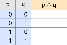
Examine the way the truth values for the atomic propositions have been laid out. As described earlier in the overview, we are listing each combination of truth values by essentially using a rotary or dial system. This ensures we list all possible combinations of truth values.
Step 4: Fill in all of the missing truth values under the desired proposition’s column
Let’s do this one row at a time. Let’s start with the first row, where $p = 0$ and $q = 0$, highlighted in this table:
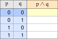
What value do we fill in to the highlighted, yellow cell? We need to refer back to the definition of conjunction: the conjunction of two propositions $p$ and $q$, denoted $p \land q$, is true only when both $p$ and $q$ are true. If either $p$ or $q$ is false, then the conjunction itself is false.
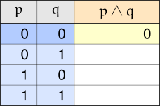
Remember that we use $0$ to represent a false truth value, and $1$ to represent a true one. In the row we’re examining, both $p$ and $q$ are false, since both are equal to $0$. Since not both $p$ and $q$ are true, $p \land q$ is false, so we write $0$ in the highlighted cell, as shown below:
This leaves us with the following partially filled out table:
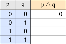
We continue on to the next row, where $p = 0$ and $q = 1$, highlighted below:
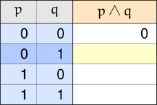
Appealing to the definition, since one of the atomic propositions is false — here, $p = 0$ — the conjunction $p \land q$ is also false. We place a $0$ in the highlighted cell, shown below:
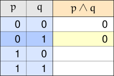
This leaves us with a slightly more filled out table, shown below:
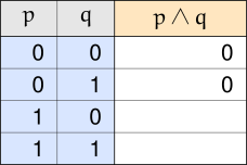
Let’s continue on and examine the third row, where $p = 1$ and $q = 0$. Here, since one of the atomic propositions is false, the conjunction $p \land q$ continues to be false, and we fill in a $0$ in the third blank cell, shown below:
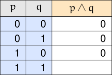
Now we are on the last row, where $p = 1$ and $q = 1$. Here, both atomic propositions are true. This means the conjunction $p \land q$ is, by definition, true. That means in this final blank cell we fill in a $1$, leaving us with the completed truth table for the conjunction $p \land q$:
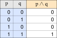
This example shows the basic procedure. From now on, we can just fill in the values as needed, without any need to repeat any of the exposition here.
We have seen how to construct a truth table from scratch. Now, it’s really just a matter of appealing to the definitions of the logical connectives in order to construct truth tables for them. Knowing the truth tables for the logical connectives is going to make working with even more complicated expressions much easier, since any complicated expression is essentially just a bunch of atomic propositions combined with the logical connectives described here.
Here, we are going to use $p$ and $q$ as the atomic propositions for the expressions.
This is a really simple truth table, since negation can operate on one proposition at a time. Remember that the negation of a proposition has the opposite truth value of the proposition itself.
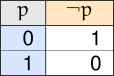
We already saw this in the example above, but we’ll show the table here for the sake of completeness.
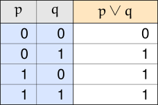
Based on the definition of disjunction, we know that if at least one of the atomic propositions is true, then the disjunction itself is also true.
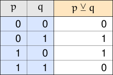
The definition essentially tells us that the exclusive-or of two atomic propositions is true whenever the atomic propositions have different truth values; or put another way, not equal to each other.
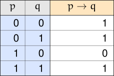
The definition of implication tells us that the only time an implication is false is if $p$ is true, and $q$ is false. Otherwise, the implication is true.
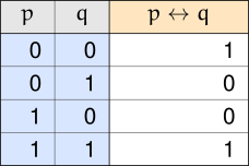
The definition for a biconditional essentially tells us that if the two atomic propositions have the same truth value, meaning they are equal to each other, then the biconditional itself is true. It is false otherwise. We can almost think of the biconditional as being the exact opposite of an exclusive-or between two propositions.
Something we can do is simply append the columns for each of the logical connectives into one big overall table. You have to be careful when doing this to make sure the rows line up with the appropriate rows for the atomic propositions. If the order of the atomic propositions differs, or if the numbering method used yields a different ordering for the combinations of truth values for the atomic propositions, the results may not be correct.
Here, we used the same ordering for the atomic propositions themselves, and the combinations of truth values for those atomic propositions. We will have to extend the negation table by an additional two rows, but again, we fill in any values needed by appealing to the definition of negation, and paying attention to the values of the atomic propositions in the row we are evaluating.
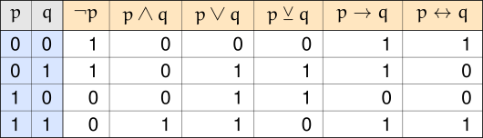
Notice that we just produced a truth table that has more than one expression column, one expression column for each of the logical connectives we use to form compound propositions.
If we are trying to determine the truth value of a complicated expression, we can do the same thing. We can identify all of the parts of the more complicated expression, and gradually build up the truth value of the final, desired expression. Doing this helps us keep track of values, preventing us from having to work out complicated expressions all at once.
We use so-called intermediary columns to hold the parts of the complicated expression that are easy to calculate. Usually, we break a complicated expression up based on where the logical connectives are. Here is an example.
Consider the expression $\neg (p \land q)$. Working out its truth value directly, row by row, means checking $p$, checking $q$, combining them with conjunction, and then negating the result — three things to keep in your head at once for every row.
An intermediary column makes this easier. We start by building a table with an intermediary column for the simpler piece, $p \land q$ — a table we already know how to construct — alongside the column for the desired expression $\neg (p \land q)$ itself, still blank:
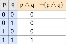
To fill in that blank column, we no longer need to think about $p$ and $q$ at all — we just take the negation of whatever is already in the $p \land q$ column, one row at a time:
\[ \begin{array}{l|l|l} p \land q & \neg (p \land q) & \text{Result} \\ \hline 0 & \neg (0) & 1 \\ 0 & \neg (0) & 1 \\ 0 & \neg (0) & 1 \\ 1 & \neg (1) & 0 \end{array} \]All we need to do now is copy the Result column from the above table into the truth table we are building.
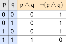
That’s the advantage of an intermediary column: instead of working out $p$, $q$, and the negation of their conjunction all at once, we break the work into two simple steps, each of which is just a single connective’s truth table.
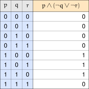
Consider the expression $p \land (\neg q \lor \neg r)$. This one has three atomic propositions — $p$, $q$, and $r$ — so its full truth table needs eight rows, and this time we’ll use more than one intermediary column.
We start with intermediary columns for the two simplest pieces, $\neg q$ and $\neg r$:
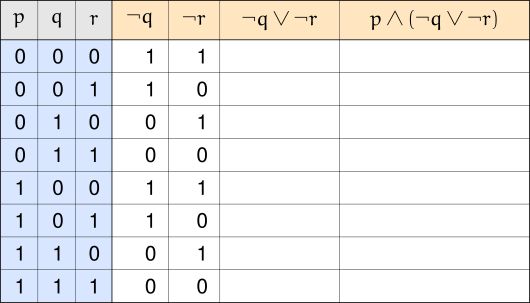
With those two columns in hand, we build a third intermediary column for $\neg q \lor \neg r$, taking the disjunction of the two columns we just built, row by row:
\[ \begin{array}{l|l|l|l} \neg q & \neg r & \neg q \lor \neg r & \text{Result} \\ \hline 1 & 1 & 1 \lor 1 & 1 \\ 1 & 0 & 1 \lor 0 & 1 \\ 0 & 1 & 0 \lor 1 & 1 \\ 0 & 0 & 0 \lor 0 & 0 \\ 1 & 1 & 1 \lor 1 & 1 \\ 1 & 0 & 1 \lor 0 & 1 \\ 0 & 1 & 0 \lor 1 & 1 \\ 0 & 0 & 0 \lor 0 & 0 \end{array} \]All we need to do now is copy the Result column from the above table into the truth table we are building.
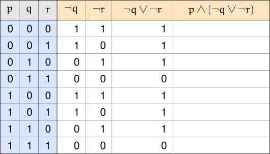
Finally, filling in $p \land (\neg q \lor \neg r)$ is just a matter of taking the conjunction of $p$ column with the $\neg q \lor \neg r$ column we just finished — no need to think about $q$ or $r$ individually at all:
\[ \begin{array}{l|l|l|l} p & \neg q \lor \neg r & p \land (\neg q \lor \neg r) & \text{Result} \\ \hline 0 & 1 & 0 \land 1 & 0 \\ 0 & 1 & 0 \land 1 & 0 \\ 0 & 1 & 0 \land 1 & 0 \\ 0 & 0 & 0 \land 0 & 0 \\ 1 & 1 & 1 \land 1 & 1 \\ 1 & 1 & 1 \land 1 & 1 \\ 1 & 1 & 1 \land 1 & 1 \\ 1 & 0 & 1 \land 0 & 0 \end{array} \]We then copy the Result column from the above table into the truth table we are building, same as usual.
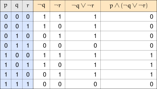
We could leave the table as it is, with a column for every intermediary piece we used along the way. Or, we could construct a condensed table that only shows the atomic propositions along with the desired expression.
Just like in the arithmetic of real numbers, there is an order we should follow when evaluating logical expressions.
For instance, in the arithmetic of real numbers, we abide by the following rules:
Using this scheme for evaluating arithmetic expressions, we do the following:
\[ \begin{align*} 2 - 3^2 \cdot (4 + 6 \div 2) &= 2 - 3^2 \cdot (4 + 3) \\ &= 2 - 3^2 \cdot 7 \\ &= 2 - 9 \cdot 7 \\ &= 2 - 63 \\ &= -61 \end{align*} \]Here we introduce a scheme to help us determine which operations should be done in order to achieve the correct final result.
Consider the following example.
There are two ways to evaluate this expression.
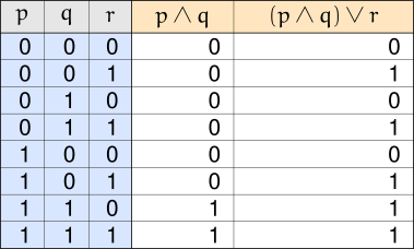
Method 1: $(p \land q) \lor r$
Method 2: $p \land (q \lor r)$
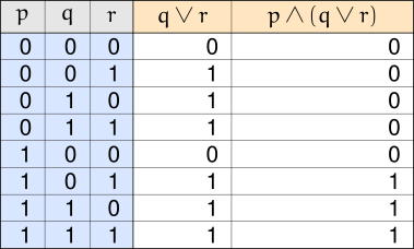
Note that from what we see,
$$(p \land q) \lor r \neq p \land (q \lor r)$$when $p = 0$, $q = 0$, $r = 1$, and when $p = 0$, $q = 1$, $r = 1$.
Based on this calculation, we see that the expression
$$p \land q \lor r$$is ambiguous — we don’t know how to evaluate it until parentheses are added, or until some order of operations is established.
The following is a commonly used scheme for an order of operations:
Using this order, we remove any ambiguity from logical expressions.
Using the previously established order of operations, we see that the expression
$$p \land q \lor r$$is equivalent to the expression
$$(p \land q) \lor r$$Suppose we had that $p = 1$, $q = 0$, $r = 1$. Then we’d have that
\[ \begin{align*} (p \land q) \lor r &= (1 \land 0) \lor 1 \\ &= 0 \lor 1 \\ &= 1 \end{align*} \]If we wanted to evaluate the disjunction first, we’d have to use parentheses, since
$$p \land (q \lor r)$$is not equivalent to the expression $p \land q \lor r$.
With the order of operations, we remove any ambiguity, and do not have to rely on parentheses unless we want to give precedence to operations lower in the order.
The final simplification reveals the final, overall truth value to be $0$.
In this book, we adopt the above order of operations, but will only make shallow use of it. Basically, what this effectively means is that we will make very liberal use of parentheses, even when they aren’t strictly necessary.
While the relative order between $\neg$, $\land$, $\lor$, $\to$, and $\leftrightarrow$ is somewhat standardized (heavy emphasis on the word “somewhat”), it is hardly universal. This is especially true when $\veebar$ is thrown into the mix.
Many texts use $()$ liberally as well. In some ways, the order of operations presented here was entirely engineered to meet this book’s needs, and this order’s scope is only contained within this book.
This is why, going forward, we will hardly rely on this order of operations, and instead opt to use the standard trick of using $()$ to indicate which operations take precedence over others.
A blank piece of paper allows one to express an idea anywhere on the page, in any arrangement. But following a chain of arithmetic is much easier when it’s laid out in a consistent, organized manner.
In this book, any arithmetic (based on real numbers, logic, or some other system) will generally be shown in a tabular format. There will be two benefits to this:
Let’s see an example.
There is a slightly different format we’ll use for expressions that don’t already appear in a large, single block.
We’ve seen plenty of primitive propositions whose truth values are fixed:
\[ \begin{array}{ll} \text{Calvin Coolidge was the 30th President of the United States of America.} & \text{(true)} \\ \\ \text{Mitochondria convert ADP into ATP via cellular respiration.} & \text{(true)} \\ \\ \text{Leonardo da Vinci painted the famous ceiling fresco in the Sistine Chapel.} & \text{(false)} \end{array} \]We’ve also seen compound propositions whose truth values depend on the truth values of its atomic propositions.
\[ \begin{array}{ll} 2+2=5 \text{ and } 2+3=6. & \text{(false)} \\ \\ \text{Parallelograms with four equal sides and four equal angles are squares.} & \text{(true)} \\ \\ \text{If an integer is prime and even, then that integer is two.} & \text{(true)} \\ \\ \text{If } x=2 \text{ or } x=3 \text{, then } x^2-5x+6=0. & \text{(true)} \end{array} \]Typically, the compound propositions we work with are made up of generic propositions that could be true, or could be false. This means we need to examine all combinations of truth values for the atomic propositions to determine the overall truth value of the compound proposition.
Of course, we usually will only be interested in compound propositions that are true. This is how we frame the upcoming discussion: when are compound propositions true?
We’ve seen some examples of compound propositions that — for some combinations of truth values — are true.
We construct a truth table. We’ll highlight the column we are interested in examining.
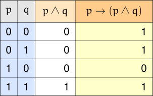
Only some of the combinations of truth values for $p$ and $q$ yield a truth value of $1$ when combined in the desired compound proposition. Those combinations are as follows: $p=0,q=0$; $p=0,q=1$; and $p=1,q=1$.
Only one combination yields a false truth value ($0$) when combined: $p=1,q=0$.
Let’s dispense with the suspense; we already know what word we’ll use to describe compound propositions that can be true.
A compound proposition is called satisfiable if there exists some combination of truth values for its atomic propositions that yield a truth value of $1$.
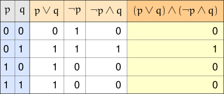
Here, we see that there is only one combination of truth values for $p$ and $q$ for where $(p \lor q) \land (\neg p \land q)$ is true, namely $p=0,q=1$.
Hence, $(p \lor q) \land (\neg p \land q)$ is satisfiable, even if just barely.
We have yet to see a proposition that is always true, no matter what combination of truth values are assigned to its atomic propositions.
We’ve seen $p \to (p \land q)$ above, but changing to the disjunction yields interesting changes.
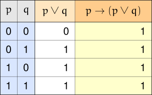
Notice that every row in the final column contains $1$.
A compound proposition is called a tautology when it is always true, no matter what truth values are taken by its atomic propositions.
Sometimes when we come across a tautology in an expression, we can replace it with the symbol $\top$ (sometimes also written $T_0$), but since the truth value is always $1$, we can always replace the expression with its truth value $1$.
It should be noted that it may preferable to either use $\top$ or $T_0$ when working with propositions, because those symbols have additional context to them than the literal value $1$. Those symbols signify that we are working with a proposition always happens to be true.
We’ve seen a proposition that is always true, but are there propositions that are never true?
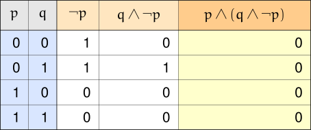
Of course, we should probably expect this proposition to always be false, because it is asserting both $p$ and $\neg p$.
You can’t assert both $p$ and $\neg p$, because they contradict each other — which leads us to our next definition.
A compound proposition is a contradiction when it is always false, no matter what truth values are assumed by its atomic propositions.
Just like with tautologies, we sometimes use the symbol $\bot$ (sometimes also written $F_0$) to represent a contradiction. But since a contradiction is always false, we can also just use $0$ — though we may prefer $\bot$ or $F_0$ if we wish to convey that we’re talking about a proposition, rather than a literal value.
At this point, we’re familiar with the fundamental unit of logic — the proposition. We’ve seen how to combine them into compound propositions, and how to use truth tables to identify propositions that are always true — tautologies.
With these tools, we are ready to start discussing the heart of logical deduction and our unique ability to reason — the Laws of Logic!
Before we dive into the deep end, let’s wade in a shallow example where we examine a few propositions that involve the biconditional connective.
As usual, we can construct a truth table showing all intermediary values.
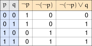
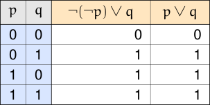
The final column resembles the truth table for the compound proposition $p \lor q$:
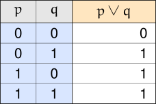
So under all the exact same circumstances (meaning, same combinations of truth values for $p$ and $q$) the expressions $\neg (\neg p) \lor q$ and $p \lor q$ have the same truth value.
Let’s examine the double negation more closely:
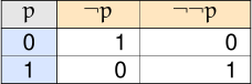
We see that $p$ and $\neg \neg p$ have the exact same truth values, regardless of what value $p$ has.
Since $p$ and $\neg \neg p$ always have the same truth values under all conditions, we can swap them out with each other in expressions, without affecting the overall truth value.
This explains why $\neg \neg p \lor q$ and $p \lor q$ have the same truth values for all combinations of truth values for $p$ and $q$; because we can swap out $\neg \neg p$ with just $p$ without affecting the truth values.
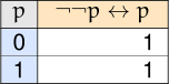
Notice that because $\neg \neg p$ and $p$ have the same truth values, we expect the biconditional connecting them to always be true — a tautology:
\[ \begin{array}{l|l|l|l|l} p & \neg p & \neg \neg p & \neg \neg p \leftrightarrow p & \text{Result} \\ \hline 0 & 1 & 0 & (0) \leftrightarrow (0) & 1 \\ 1 & 0 & 1 & (1) \leftrightarrow (1) & 1 \end{array} \]It is as expected:
Furthermore,
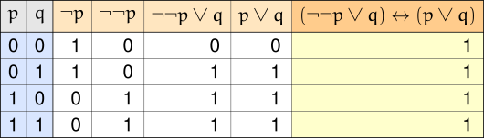
So we see that $(\neg \neg p \lor q) \leftrightarrow (p \lor q)$ is a tautology. We prefer $p \lor q$, since it’s a simpler expression than $\neg \neg p \lor q$.
In the previous example we saw how — when the biconditional between two propositions is a tautology — we can essentially just swap out one expression that has the same behavior under its atomic propositions for another, without changing the overall truth value.
Let’s see another example.
We may suspect that the order we list the atomic propositions in a disjunction may not actually matter, but we can easily verify this with a truth table:
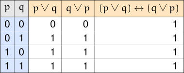
So we now see that whenever we see a disjunction between two propositions, we can swap the order without affecting the truth value.
Let’s see one more example of some “equivalent” expressions.
Again, let’s organize our results into a truth table:
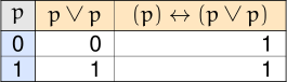
Based on this example, we now know that if we ever see a proposition disjunctioned with itself, we can just replace the entire disjunction with a single copy of the atomic proposition used.
We just saw three examples of biconditionals that were tautologies. A reasonable next question would be “so what?”
This proposition uses the three kinds of propositions we saw in the three previous examples. We can probably guess where this example is leading, but let’s continue on.
We’ve kept parentheses around every grouping here on purpose. We haven’t justified anything about rearranging parentheses yet — only swapping the order of a disjunction’s two sides, and collapsing a disjunction with itself — so we’ll stick to those two moves and keep checking our work with a truth table at every step.
We suspect we can replace $\neg \neg p$ with just $p$, like so, without affecting the overall truth value:

So we can still replace $\neg \neg p$ with just $p$ and still get the same truth values:
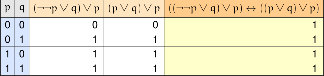
Let’s continue examining $(p \lor q) \lor p$ instead.
Previously we also saw that in a disjunction, we could swap the propositions without affecting the overall truth value. Let’s see if we can swap out $p \lor q$ for $q \lor p$ without affecting the truth value:
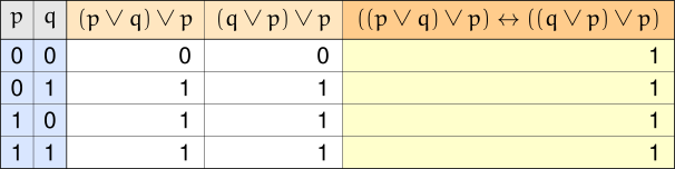
Ok, we still get the same truth values under the same combinations of truth values for $p$ and $q$.
Let’s keep rearranging things this way, still checking our work with a truth table at every step, until the two copies of $p$ end up sitting right next to each other:
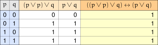
We also saw that we could replace a disjunction between a proposition and itself with just that proposition. Since $(p \lor p)$ behaves just like $p$, this leaves us with $p \lor q$ — matching what the table above already confirms.
Hence we see that
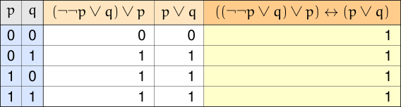
Meaning the proposition $((\neg \neg p \lor q) \lor p) \leftrightarrow (p \lor q)$ is a tautology. Both $(\neg \neg p \lor q) \lor p$ and $(p \lor q)$ have the exact same behavior under all combinations of truth values for $p$ and $q$.
In essence, what this means is that whenever we encounter the expression $(\neg \neg p \lor q) \lor p$, we can fully understand it by examining $(p \lor q)$ instead — we can basically just replace $(\neg \neg p \lor q) \lor p$ with $(p \lor q)$ without affecting anything.
Being as $(p \lor q)$ is much simpler than $(\neg \neg p \lor q) \lor p$ — without all the extra copies of the $\neg$ symbol, the extra $\lor$ symbols, or the extra copy of proposition $p$ — we’d rather work with the expression $(p \lor q)$.
The past couple of examples have demonstrated how complicated expressions can be replaced (and better understood) with simpler expressions.
The reason why we can replace a complicated proposition with a simpler proposition is because that simpler proposition exhibits the exact same behavior as the more complicated proposition when the atomic propositions assume — or take — the same combination of truth values. By “the same behavior,” we mean they have the same truth values, meaning the biconditional is a tautology.
Two propositions $S_1$ and $S_2$ are called logically equivalent, and we write
$$S_1 \Longleftrightarrow S_2$$whenever the biconditional
$$S_1 \leftrightarrow S_2$$is a tautology.
At least one of $S_1$ and $S_2$ needs to be compound for this to be interesting. We actually already saw an example where only one side was: $\neg \neg p$ is logically equivalent to just $p$, even though $p$ itself is primitive. Comparing two primitive propositions to each other isn’t nearly as useful — a primitive proposition’s truth value doesn’t depend on the truth value of any other proposition, so there’s no combination of truth values to check across.
Logical equivalence is the basis for the Laws of Logic.
The Laws of Logic are nothing more than a list of logical equivalencies.
Here, we present a rather long list of known logical laws.
| Law of Double Negation | $\neg \neg p \Longleftrightarrow p$ |
| DeMorgan’s Laws | $\begin{array}{c} \neg (p \land q) \Longleftrightarrow \neg p \lor \neg q \\ \neg (p \lor q) \Longleftrightarrow \neg p \land \neg q \end{array}$ |
| Commutative Laws | $\begin{array}{c} p \land q \Longleftrightarrow q \land p \\ p \lor q \Longleftrightarrow q \lor p \end{array}$ |
| Associative Laws | $\begin{array}{c} (p \land q) \land r \Longleftrightarrow p \land (q \land r) \\ (p \lor q) \lor r \Longleftrightarrow p \lor (q \lor r) \end{array}$ |
| Distributive Laws | $\begin{array}{c} p \land (q \lor r) \Longleftrightarrow (p \land q) \lor (p \land r) \\ p \lor (q \land r) \Longleftrightarrow (p \lor q) \land (p \lor r) \end{array}$ |
| Idempotent Laws | $\begin{array}{c} p \land p \Longleftrightarrow p \\ p \lor p \Longleftrightarrow p \end{array}$ |
| Identity Laws | $\begin{array}{c} p \land T_0 \Longleftrightarrow p \\ p \lor F_0 \Longleftrightarrow p \end{array}$ |
| Inverse Laws | $\begin{array}{c} p \land \neg p \Longleftrightarrow F_0 \\ p \lor \neg p \Longleftrightarrow T_0 \end{array}$ |
| Domination Laws | $\begin{array}{c} p \land F_0 \Longleftrightarrow F_0 \\ p \lor T_0 \Longleftrightarrow T_0 \end{array}$ |
| Absorption Laws | $\begin{array}{c} p \land (p \lor q) \Longleftrightarrow p \\ p \lor (p \land q) \Longleftrightarrow p \end{array}$ |
Just like we did in the examples, all of the above can be verified by examining a truth table containing a biconditional and determining whether or not the biconditional is a tautology.
There are a couple more logical equivalencies that prove to be useful.
| Law of Material Implication | $p \to q \Longleftrightarrow \neg p \lor q$ |
| Law of Material Equivalence | $p \leftrightarrow q \Longleftrightarrow (p \land q) \lor (\neg p \land \neg q)$ |
| Exclusive-or Equivalence | $p \veebar q \Longleftrightarrow (p \land \neg q) \lor (\neg p \land q)$ |
| Law of Mutual Implication | $p \leftrightarrow q \Longleftrightarrow (p \to q) \land (q \to p)$ |
| Negated Biconditional Equivalence | $p \veebar q \Longleftrightarrow \neg (p \leftrightarrow q)$ |
In the previous section we saw an example where we used tautologically true biconditionals to “simplify” complicated propositional expressions into simpler propositional expressions. Whatever we could say about the simpler expressions could also be said about their more complicated, logically equivalent counterparts (except perhaps our preference for working with the simpler expressions, of course).
In this section we do more work with logical equivalencies, similar to what we saw in the examples seen previously. Our work here will bear a striking resemblance to our experience in dealing with the arithmetic and algebra of real numbers. In fact, the upcoming work we are about to engage with has been dubbed the “algebra of propositions.”
In the previous example, we saw how to take a complicated proposition and produce a simpler proposition that always had the same truth value.
Now that we have a big list of logical equivalencies under our belt, we can see how to use those equivalencies to more quickly find equivalent propositions, rather than trudge through truth tables all the time.
Previously, we made guesses about how the following propositions were related to each other:
\[ \begin{align*} & \neg \neg p \text{ compared to } p \\ & p \lor q \text{ compared to } q \lor p \\ & p \lor p \text{ compared to } p \end{align*} \]and used what we found to make a bunch of truth tables, which is reviewed below:
\[ \begin{align*} \neg \neg p &\Longleftrightarrow p \\ p \lor q &\Longleftrightarrow q \lor p \\ p \lor p &\Longleftrightarrow p \end{align*} \]Instead of using truth tables, let’s just use the laws of logic.
\[ \begin{array}{ll} (\neg \neg p \lor q) \lor p \Longleftrightarrow (p \lor q) \lor p & \text{by the Law of Double Negation} \\ (p \lor q) \lor p \Longleftrightarrow (q \lor p) \lor p & \text{by the Commutative Law of } \lor \\ (q \lor p) \lor p \Longleftrightarrow q \lor (p \lor p) & \text{by the Associative Law of } \lor \\ q \lor (p \lor p) \Longleftrightarrow q \lor p & \text{by the Idempotent Law of } \lor \\ q \lor p \Longleftrightarrow p \lor q & \text{by the Commutative Law of } \lor \end{array} \]We probably could have used fewer steps by more carefully applying the commutative and associative laws, but regardless, we arrived at the same proposition as we did in Example 1.5.4.
Let’s turn our sights to a new example we haven’t seen before, and compare using truth tables to using logical equivalencies.
We’re interested in seeing if there’s a simpler, equivalent way of writing an expression like $\neg (p \to q)$ — one that doesn’t use the implication, but is instead just a combination of conjunctions, disjunctions, and negations. First, let’s construct a truth table for $\lnot (p \rightarrow q)$:
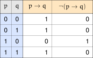
Suppose we didn’t know about the Laws of Logic. How can we proceed? We notice that there is only one $1$ in the column for $\neg (p \to q)$. We may remember that the conjunction of $p$ and $q$ also only has one $1$ as well.
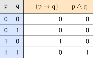
However, the $1$s aren’t in the same row. Notice that if we swap the $1$s and $0$s in the $q$ column, we can get the $1$s to line up with those for $p$. But how do we swap $1$s and $0$s of a proposition?
We negate it! Let’s add $\neg q$ to the table.
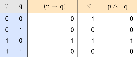
Now we see that $\neg (p \to q)$ and $p \land \neg q$ have the same truth values for all combinations of truth values, meaning
$$[\neg (p \to q)] \leftrightarrow [p \land \neg q]$$is a tautology.
Thus, we see that
$$[\neg (p \to q)] \Longleftrightarrow [p \land \neg q]$$Using the truth table method required us to make keen observations on how to work, manipulate, and coax truth values into the proper rows so they line up.
What if we don’t see a way to make values line up? Fortunately, there is a way we can avoid relying on our ability to make clever observations: we use the Laws of Logic!
Let’s use the Laws of Logic we have seen to try and come up with a logically equivalent proposition:
\[ \begin{array}{lll} & \boldsymbol{\neg (p \to q)} & \textbf{Reason} \\ \Longleftrightarrow & \neg (\neg p \lor q) & \text{Law of Material Implication} \\ \Longleftrightarrow & \neg \neg p \land \neg q & \text{DeMorgan's Law} \\ \Longleftrightarrow & p \land \neg q & \text{Law of Double Negation} \end{array} \]This is the same proposition we got by using truth tables! We just used logical equivalencies we were familiar with, instead of a keen eye (which may have blind spots). There was also a lot less work involved too!
In the previous example, we listed the logical equivalencies on separate lines, citing the logical law being appealed to. This is certainly a fine way to organize one’s work, and has its advantages.
In this book, we opt to use a tabular format to organize our work, unless the occasion calls for some other format. We adopt a three-column format:
\[ \begin{array}{lll} \Longleftrightarrow & \text{Propositional Expression} & \text{Reason} \end{array} \]We can demonstrate this format using the same proposition from the previous example.
Notice that we skip the first row in the left column. We also use bold font for the first row.
We’ve seen a couple of examples where we use a couple of logical laws. Some examples require more laws to simplify.
One thing to notice is that initially, we had four atomic propositions: $p$, $q$, $r$, and $s$. After all of our work above, we ended up with only two: $p$ and $r$. This means that the large, complicated compound proposition’s truth value actually is unaffected by $q$ or $s$. The truth value is driven, or affected, only by $p$ and $r$.
While the content we’ve seen so far seems ethereal, with little application outside of simplifying logical propositions, logic dictates almost every avenue of study. In our everyday lives, we like to think our actions are reasonable and make sense. Certainly, we can use logic to analyze a situation so we can maximize our profit from it, whether our profit is in the form of friendship, promotions at work, happiness, health, or money.
One such application of logic has had a profound impact on human history. In 1938, a paper “A Symbolic Analysis of Relay and Switching Circuits” was published. In that paper, author Claude Shannon showed that Boolean Logic (what we’ve been studying so far in this book) can be used to simplify the design of relay circuits that were used in the construction of electromechanical devices back in the day. (Likewise, these relay circuits could be used to solve Boolean algebra problems, essentially meaning that relay circuits are equivalent to Boolean/propositional expressions.)
This insight paved the way for future computer advancements, culminating in the development of modern computer chip designs, including modern CPU, GPU, and now TPU chip designs.
In this section, we take a look at a very basic framework for taking “complicated” circuits and producing equivalent, simpler circuits.
An electrical circuit at its core is simply a network of switches that are designed to allow or block electricity from flowing from one terminal to another.
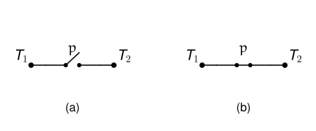
Here is the simplest switching network:
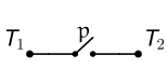
Here, $T_1$ is the starting terminal, and $T_2$ is the ending terminal. Electrical current is applied at $T_1$.
Here, there is one switch, labeled $p$. In the diagram above, $p$ is “open,” meaning it isn’t allowing electricity to flow through.
Here is the same circuit, with switch $p$ “closed,” thus allowing electricity to flow:
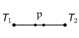
The connection between these circuits and logic is this: open switches correspond to false propositions, and closed switches correspond to true propositions.
So, the first circuit we saw corresponds to when $p$ represents a false proposition ($p = 0$). The second circuit corresponds to when $p$ represents a true proposition ($p = 1$).
Here we start by showing two circuits that are used to construct more elaborate circuits.
Here is the first:
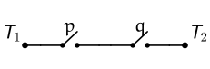
In order for electricity to flow from terminal $T_1$ to terminal $T_2$, both switches $p$ and $q$ must be closed ($p = 1$ and $q = 1$).
This is exactly the same as saying $p \land q$: when either $p$ or $q$ is open (equal to $0$), then there isn’t a connected path from $T_1$ to $T_2$. When both are closed (equal to $1$), then there is a path from $T_1$ to $T_2$.
This circuit is called the “Series Circuit” and corresponds to the conjunction operator.
Here is the second fundamental type of circuit: the “Parallel Circuit”
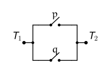
Here, we see that as long as at least one of $p$ or $q$ is closed (at least one of $p$ or $q$ is equal to $1$), then electricity can flow from $T_1$ to $T_2$.
Of course, saying $p$ or $q$ must be closed is equivalent to the disjunction of $p$ and $q$: when $p \lor q = 0$, electricity can’t flow from $T_1$ to $T_2$. When $p \lor q = 1$, electricity can flow.
From just these two circuits, we can build up many useful circuits.
The ability to simplify circuits relies on our ability to model a given circuit as a proposition containing a combination of atomic propositions, negations, conjunctions, and disjunctions.
We do that by identifying the series and parallel circuits being used in the given circuit.
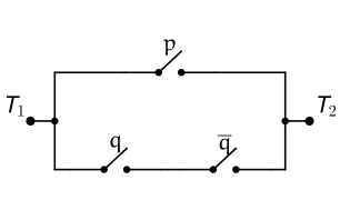
This is a parallel circuit between a single switch $p$ and a series circuit consisting of $q$ and $\neg q$.
Thus, we model this circuit as
$$p \lor (q \land \neg q)$$Now, we can use the laws of logic to simplify this proposition:
\[ \begin{array}{lll} & \boldsymbol{p \lor (q \land \neg q)} & \textbf{Reason} \\ \Longleftrightarrow & p \lor F_0 & \text{Inverse Law of } \land \\ \Longleftrightarrow & p & \text{Identity Law} \end{array} \]So, we can simplify $[p \lor (q \land \neg q)]$ to just $p$. The circuit for $p$ is below:
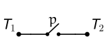
We have just produced a circuit that is equivalent to the circuit we were given, but is much simpler:
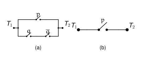
We can take a more complicated circuit and do the same thing:
Consider the following circuit:
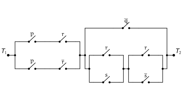
There are two sub-circuits connected in series:
$$[\quad] \land [\quad]$$The first part is a parallel circuit consisting of a series circuit along each branch:
$$[(p \land r) \lor (p \land \neg r)] \land [\quad]$$The second sub-circuit consists of another parallel circuit, the second branch of which is more complicated:
$$[(p \land r) \lor (p \land \neg r)] \land [(\neg q) \lor [(r \lor s) \land (r \lor \neg s)]]$$Now that we have the underlying proposition, we can simplify:
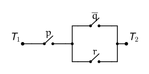
\[ \begin{array}{lll} & \boldsymbol{[(p \land r) \lor (p \land \neg r)] \land [(\neg q) \lor [(r \lor s) \land (r \lor \neg s)]]} & \textbf{Reason} \\ \Longleftrightarrow & [p \land (r \lor \neg r)] \land [(\neg q) \lor [(r \lor s) \land (r \lor \neg s)]] & \text{Distributive Law} \\ \Longleftrightarrow & [p \land T_0] \land [(\neg q) \lor [(r \lor s) \land (r \lor \neg s)]] & \text{Inverse Law} \\ \Longleftrightarrow & p \land [(\neg q) \lor [(r \lor s) \land (r \lor \neg s)]] & \text{Identity Law} \\ \Longleftrightarrow & p \land [(\neg q) \lor [r \lor (s \land \neg s)]] & \text{Distributive Law} \\ \Longleftrightarrow & p \land [(\neg q) \lor [r \lor F_0]] & \text{Inverse Law} \\ \Longleftrightarrow & p \land [(\neg q) \lor r] & \text{Identity Law} \end{array} \]This final proposition doesn’t seem to admit any further simplifications using the laws of logic at our disposal.
As such, we accept this final proposition for our simplified circuit:
Something we could do, if we were worried someone may take our circuit designs, is to obfuscate them by taking a simple circuit and using the laws of logic “in reverse,” so to speak, to produce an equivalent, more complicated circuit.
A deranged mad man is planning to abduct a group of people and force them to solve a series of puzzles to survive.
One such puzzle involves opening and closing a network of valves designed to carry a liquid antidote to a poison the mad man will administer to his victims. If the kidnapped individuals can configure the valves in a satisfiable way, the liquid antidote will be carried through the plumbing network to vials the victims can drink from.
Initially, the mad man starts with just
$$p \land q$$but wants to design a more complicated network to hide the simplicity, so the lunatic uses the laws of logic in the following way:
\[ \begin{array}{lll} & \boldsymbol{p \land q} & \textbf{Reason} \\ \Longleftrightarrow & p \land (q \land T_0) & \text{Identity Law} \\ \Longleftrightarrow & p \land (q \land (r \lor \neg r)) & \text{Inverse Law} \\ \Longleftrightarrow & p \land [(q \land r) \lor (q \land \neg r)] & \text{Distributive Law} \\ \Longleftrightarrow & [p \land (q \land r)] \lor [p \land (q \land \neg r)] & \text{Distributive Law} \\ \Longleftrightarrow & [(p \lor F_0) \land (q \land r)] \lor [p \land (q \land \neg r)] & \text{Identity Law} \\ \Longleftrightarrow & [(p \lor (s \land \neg s)) \land (q \land r)] \lor [p \land (q \land \neg r)] & \text{Inverse Law} \\ \Longleftrightarrow & [((p \lor s) \land (p \lor \neg s)) \land (q \land r)] \lor [p \land (q \land \neg r)] & \text{Distributive Law} \\ \Longleftrightarrow & [(p \lor \neg s) \land (q \land r) \land (p \lor s)] \lor [p \land (q \land \neg r)] & \text{Commutative Law} \\ \Longleftrightarrow & [(p \lor \neg s) \land (q \land r) \land (p \lor s)] \lor [q \land \neg r \land p] & \text{Commutative Law} \end{array} \]So essentially, we started with the following plumbing circuit:
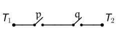
and constructed the following circuit:
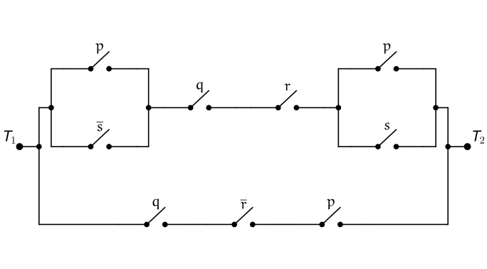
The mad man is pleased with his new design, and implements it for his plan. Or he would have, had he not been caught by investigators for his recent tax fraud schemes.
In the previous example, we saw how the laws of logic can be used to turn simple propositions into more complex ones. For example, a combination of the identity laws and inverse laws allow us to introduce superfluous atomic propositions.
We also saw that propositions can be used to model non-electric networks as well, such as a valved plumbing network. Any kind of gated network can be modeled as a proposition.
All of the propositions we’ve dealt with so far have had definite truth values. For example,
$$\text{Thomas Jefferson was the second president of the United States.}$$is a proposition that is known to be false. A statement such as
$$\text{2 + 2 = 4, or 2 + 2 = 5.}$$is a compound proposition that is true.
However, a statement such as
$$\text{$n$ is 1 more than a multiple of 3.}$$is not a proposition, because we don’t know whether it’s true or false. We would need to know the value of $n$ in order to reach such a conclusion. For example, the statement is false when $n = 5$, but true when $n = 16$. Here, we’ll deal with sentences involving variables like this one.
Consider the statement
$$x + 3 = 8.$$Here, we aren’t asking what value of $x$ solves the equation (we could, but that isn’t our focus). Instead, we’re asking whether, given a specific value of $x$, the statement is a true proposition or a false proposition.
We start by modeling the statement using a letter, like we’ve done up to this point, but we also use parentheses to denote the variable $x$:
\[ \begin{array}{rl} p(x)\text{: } &x + 3 = 8. \end{array} \]We can substitute values in for $x$ to get different propositions:
\[ \begin{array}{rl} p(5)\text{: } &5 + 3 = 8 \\ p(3)\text{: } &3 + 3 = 8 \\ p(-4.73)\text{: } &-4.73 + 3 = 8 \end{array} \]We can evaluate some of these propositions:
\[ \begin{array}{ll} p(5) &= 1 \\ p(3) &= 0 \\ p(-4.73) &= 0 \end{array} \]Consider the statement
\[ \begin{array}{rl} p(x)\text{: } &x \text{ was the 30th president of the United States.} \end{array} \]We can evaluate this statement with many values substituted in for $x$:
\[ \begin{array}{ll} p(\text{James K. Polk}) &= 0 \\ p(\text{Cecil Rhodes}) &= 0 \\ p(\text{Grover Cleveland}) &= 0 \\ p(\text{Calvin Coolidge}) &= 1 \\ p(\text{Bill Clinton}) &= 0 \end{array} \]Both of these examples are open statements — sentences with variables whose truth value can’t be pinned down until we substitute something in for those variables.
An open statement is any declarative sentence that has one or more variables, and thus is not a proposition, but becomes a proposition after values are substituted for all of its variables.
Just like with ordinary propositions, we write $p(x) = 0$ if the value of $x$ makes $p(x)$ a false proposition, and $p(x) = 1$ if the value of $x$ makes $p(x)$ a true proposition.
A statement $p(x)$ that represents an open statement with variable $x$ is often called a propositional function.
A propositional function can depend on more than one variable, as the next example demonstrates.
The U.S. Postal Service will only ship a package in a box that meets certain requirements: the sum of the box’s length and girth must not exceed 108 inches, where the girth is the perimeter of the box’s rectangular cross section.
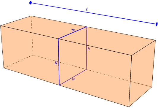
Letting $\ell$, $w$, and $h$ represent a box’s length, width, and height respectively, the perimeter of that cross section is $2w + 2h$. So, to comply with USPS shipping requirements, we need
$$\ell + 2w + 2h \leq 108 \text{ inches.}$$We can model this situation using a propositional function with three variables:
\[ \begin{array}{rl} s(\ell, w, h)\text{: } &\ell + 2w + 2h \leq 108 \text{ inches.} \end{array} \]Can we ship a box with dimensions $\ell = 32$ inches, $w = 16$ inches, and $h = 18$ inches?
\[ \begin{array}{lll} \boldsymbol{s(32, 16, 18)} & = & (32) + 2(16) + 2(18) \leq 108 \\ & = & 32 + 32 + 36 \leq 108 \\ & = & 100 \leq 108 \\ & = & 1 \end{array} \]Because $100 \leq 108$, we have $s(32, 16, 18) = 1$, so we can ship a box with these dimensions.
What about a box with dimensions $\ell = 20$ inches, $w = 18$ inches, and $h = 30$ inches?
\[ \begin{array}{lll} \boldsymbol{s(20, 18, 30)} & = & (20) + 2(18) + 2(30) \leq 108 \\ & = & 20 + 36 + 60 \leq 108 \\ & = & 116 \leq 108 \\ & = & 0 \end{array} \]Since $116 \not\leq 108$, we can’t ship a box with length $20$ inches, width $18$ inches, and height $30$ inches with USPS.
Let’s reconsider the president example.
For the propositional function
\[ \begin{array}{rl} p(x)\text{: } &x \text{ was the 30th president of the United States,} \end{array} \]we could argue $p(3)$ is either false or undefined. We can eliminate this ambiguity by specifying what kinds of values we’re allowed to substitute into $p(x)$. If a value $a$ is allowed as an input, then $p(a)$ is either true or false. If a value $b$ is not allowed, then $p(b)$ is undefined.
Let’s restrict the values allowed as inputs to $p(x)$ to proper names. This means values like “James K. Polk,” “Cecil Rhodes,” “Grover Cleveland,” “Calvin Coolidge,” and “Bill Clinton” can be substituted for $x$ and will yield true or false.
However, when substituting a value for $x$ that isn’t a proper name, we’ll say $p(x)$ is undefined. Since $3$ isn’t a proper name, $p(3)$ is undefined.
We could further restrict the inputs to be names of U.S. presidents only, rather than just any proper name. In that case, $p(\text{Cecil Rhodes})$ would be undefined, since “Cecil Rhodes” isn’t the name of any U.S. president.
Reconsider the propositional function
\[ \begin{array}{rl} p(x)\text{: } &x \text{ was the 30th president of the United States.} \end{array} \]Suppose we restrict the allowable values to names of U.S. presidents, except “Calvin Coolidge.” Then $p(\text{Calvin Coolidge})$ would be undefined. Substituting any other U.S. president’s name yields $0$, since only Calvin Coolidge was the 30th U.S. president. Under this restriction, $p(x)$ never yields $1$ — only $0$, or undefined.
Restricting the allowable names to Spanish monarchs would also only ever yield $0$ or undefined, since no Spanish monarch was ever the 30th president of the United States. We could similarly restrict the allowable values to even integers — again, $p(x)$ would always be either false, or undefined.
Reconsider the propositional function
\[ \begin{array}{rl} p(x)\text{: } &x + 3 = 8. \end{array} \]If we restrict our inputs to integers only, we can make $p(x)$ true by substituting $5$ in for $x$. Any other integer yields $0$. Non-integers yield undefined values, since they aren’t allowed as inputs — so $p(3.14159265)$ is undefined.
However, if we restrict allowed inputs to any real number, $p(3.14159265)$ is no longer undefined — it’s equal to $0$.
The previous examples show that restricting the allowable inputs of a propositional function can greatly affect the truth values it yields. This collection of allowable values has a special name, and knowing what it consists of is vitally important.
For a given propositional function $p(x)$, the collection of values allowed to be substituted in for $x$ is called the universe of discourse, or just universe for short.
The universe is typically denoted $\mathcal{U}$, though other symbols may be used.
Consider the propositional function
\[ \begin{array}{rl} r(x)\text{: } &x \text{ has a right angle,} \end{array} \]with universe of discourse $\mathcal{U}$ the collection of all planar polygons.
Since the number $2$ isn’t a planar polygon, $r(2)$ is undefined.
Suppose $s_1$ represents a square with side length $1$. $s_1$ is a planar polygon, meaning $r(s_1)$ is either $0$ or $1$. Since every square has a right angle, $r(s_1) = 1$.
Suppose $s_2$ represents an equilateral triangle with side length $1$. $s_2$ is also a planar polygon. Since no equilateral triangle has a right angle, $r(s_2) = 0$.
As demonstrated earlier, a propositional function can have many variables — we’d need to specify the universe of discourse that all of those variables have to adhere to.
Consider the propositional function
\[ \begin{array}{rl} e(x, y)\text{: } &x + y \text{ is an even integer,} \end{array} \]with universe of discourse $\mathcal{U}$ for both $x$ and $y$ the integers. This means both $x$ and $y$ must be integers.
We’d have $e(2, 4) = 1$, $e(3, 7) = 1$, $e(1, 2) = 0$, and $e(4, 13) = 0$.
$e(2, 2.3)$, $e(2.18, 3.14)$, and $e(4.411, 10)$ would all be undefined, since $2.3$, $2.18$, $3.14$, and $4.411$ aren’t integers.
$e(2, \text{Monday})$ would also be undefined, since “Monday” isn’t an integer. Similarly, $e(\text{Red}, \text{Cactus})$ would also be undefined.
For $e(x, y)$ to yield $0$ or $1$, both $x$ and $y$ need to be integers.
It’s also possible to specify a separate universe for every variable in a propositional function.
Consider the propositional function
\[ \begin{array}{rl} q(x, y)\text{: } &x \div y \text{ is larger than 5.2,} \end{array} \]with universe for $x$, denoted $\mathcal{U}_x$, all real numbers, and universe for $y$, denoted $\mathcal{U}_y$, all real numbers except $0$.
Here, $q(2.2, 0.0001) = 1$, $q(10, 2) = 0$, $q(0.52, 0.01) = 1$, and $q(0.52, 0.1) = 0$.
$q(1, 0)$ would be undefined, since $0 \notin \mathcal{U}_y$.
$q(\text{Monday}, 1)$ would be undefined, since $\text{Monday}$ is not a real number.
$q(\text{Friday}, 0)$ would be undefined, since $\text{Friday}$ is not a real number, and $0$ is not a non-zero real number.
Of course, it’s also possible for some of a propositional function’s variables to share a universe of discourse, while others have some other universe.
Consider the propositional function
\[ \begin{array}{rl} q(x, y, z)\text{: } &(x + y) \div z = 1, \end{array} \]with universe for $x$ and $y$, denoted $M$, all integers, and universe for $z$, denoted $N$, all real numbers except $0$.
We have $q(1, 0, 1) = 1$, $q(-2, 7, 5) = 1$, $q(-1, 1, 1) = 0$, and $q(10, -23, 2) = 0$.
$q(0.1, 1, 1)$ is undefined, since the supplied value for $x$ ($0.1$) isn’t in $M$.
Similarly, $q(23, -3.14, 10)$ is undefined, since the supplied value for $y$ ($-3.14$) isn’t in $y$’s universe, $M$.
Finally, $q(20, -10, 0)$ is undefined, since the supplied value for $z$ ($0$) isn’t in $z$’s universe, $N$.
Consider the following propositional functions, both defined on the universe $\mathcal{U}$ of all integers:
\[ \begin{array}{rl} s(n)\text{: } &n^2 \text{ is even.} \\ t(m, n)\text{: } &m^2 - n^2 \text{ is even.} \end{array} \]We can find values of $n$ that make $s(n)$ true, such as $n = -4$. We can also find values of $n$ that make $s(n)$ false, such as $n = 13$. The same is true of $t(m, n)$: the values $m = 3$ and $n = -7$ make $t(m, n)$ true, while $m = 4$ and $n = -1$ make $t(m, n)$ false.
Now consider the following statements:
\[ \begin{array}{rl} \alpha\text{: } &\text{For some } n \text{, } s(n) \text{ is true.} \\ \beta\text{: } &\text{For all } m \text{ and all } n \text{, } t(m, n) \text{ is true.} \end{array} \]$\alpha$ and $\beta$ aren’t open statements, even though variables show up in them. The difference is that each statement is making a specific claim, and the truth value of that claim doesn’t depend on the values taken by the variables.
Statement $\alpha$ is claiming that some specific integer exists that makes $s(n)$ true. As we saw above, one such value is $n = -4$, so $\alpha$ is a true proposition. It doesn’t matter that $n = 13$ makes $s(n)$ false — $\alpha$ is only claiming that some satisfying value exists, and we already found one.
Likewise, $\beta$ is making a specific claim: that every single value of $m$ and every single value of $n$ makes $t(m, n)$ true. We saw that $t(m, n)$ is false when $m = 4$ and $n = -1$. Because it isn’t true that every $m$ and every $n$ make $t(m, n)$ true, $\beta$ is a false statement — regardless of the fact that some values of $m$ and $n$ do make $t(m, n)$ true.
We explore these kinds of statements here, and in the next couple of sections.
The phrases “for some $n$” (used in statement $\alpha$) and “for all $m$ and all $n$” (used in statement $\beta$) are said to quantify the propositional functions $s(n)$ and $t(m, n)$.
The following phrases are all equivalent, and specify the existential quantifier:
The phrase “for some $x$,” specifying that at least one value of $x$ exists that satisfies some condition, is called the existential quantifier.
The existential quantifier can be expressed symbolically as $\exists x$.
For any propositional function $p(n)$, we can consider the statement
$$\exists n\ p(n)$$which is equivalent to the statement “For some $n$, $p(n)$,” which in turn is equivalent to saying “For some $n$, $p(n)$ is true.” Note that in the first two phrasings, we omit the “is true” part — it’s assumed that we’re considering the existence of values of $n$ that make $p(n)$ true. We could also consider the existence of values of $n$ that make $p(n)$ false, by considering the statement
$$\exists n\ \neg p(n).$$Similarly, we can use logical connectives along with the existential quantifier. So for propositional functions $x(n)$ and $y(n)$, we can consider the statements
\[ \begin{align*} &\exists n\ [x(n) \land y(n)] \\ &\exists n\ [x(n) \lor y(n)] \\ &\exists n\ [x(n) \veebar y(n)] \\ &\exists n\ [x(n) \to y(n)] \\ &\exists n\ [x(n) \leftrightarrow y(n)] \end{align*} \]where we enclose the propositional functions in brackets to specify that the existential quantifier applies to the whole logical connective. This is different from the statements
\[ \begin{align*} &\exists n\ [x(n)] \land y(n) \\ &\exists n\ [x(n)] \lor y(n) \\ &\exists n\ [x(n)] \veebar y(n) \\ &\exists n\ [x(n)] \to y(n) \\ &\exists n\ [x(n)] \leftrightarrow y(n) \end{align*} \]where the existential quantifier only applies to the propositional function $x(n)$. In general, it’s a good idea to enclose whatever statement you want a quantifier applied to in brackets.
At this point, it’s worth pointing out that $p(x)$ is an open statement, whose truth value can only be determined after substituting in a value for $x$ from some universe of discourse, whereas $\exists n\ p(n)$ is not an open statement — it has a definite truth value (either some value of $x$ from the universe exists such that $p(x) = 1$, or no such value exists).
It’s also worth pointing out that when we say something like $\exists n\ p(n) = 1$, we mean that the statement $\exists n\ p(n)$ is equal to $1$ — we are not simply saying that $p(n) = 1$ (again, because $p(n)$ is an open statement, we’d have to substitute a value in for $n$ before we know whether $p(n) = 0$ or $p(n) = 1$).
Remember that, by definition, a statement such as $\exists n\ p(n)$ is true if we can find at least one value of $n$ that makes $p(n) = 1$. There could be infinitely many such values, $1000$ values, $10$ values, or even exactly $1$ value — the existence of at least one such value is enough to make $\exists n\ p(n)$ a true statement.
Consider the universe of all real numbers, along with the following open statements:
\[ \begin{array}{rl} p(x)\text{: } &x \geq 0 \\ q(x)\text{: } &x^2 \geq 0 \\ r(x)\text{: } &1 - x^2 = 0 \\ s(x)\text{: } &x^2 - 3x + 2 > 0 \end{array} \]The statement $\exists x\ [p(x) \land r(x)]$ is true, because there exists at least one value of $x$ ($x = 1$) that makes both $p(x) = 1$ and $r(x) = 1$. We can translate this statement as “There exists a value of $x$ such that $x \geq 0$ and $1 - x^2 = 0$.”
The statement $\exists x\ [p(x) \to q(x)]$ is true, because there exists at least one value of $x$ ($x = -1$) such that $p(x) = 0$, $q(x) = 1$, and $0 \to 1$ is true. Another value that makes this statement true is $x = 5$, since $p(5) = 1$, $q(5) = 1$, and $1 \to 1$ is true. We can translate this statement as “There exists at least one value of $x$ such that if $x \geq 0$, then $x^2 \geq 0$.”
The statement $\exists x\ [r(x) \lor s(x)]$ is true, because there exists a value of $x$ (such as $x = 4$) where $r(x) \lor s(x) = 1$, since $r(4) = 0$ and $s(4) = 1$. We can translate this statement as “There exists a value of $x$ such that $1 - x^2 = 0$, or $x^2 - 3x + 2 > 0$.”
Showing that an existentially quantified statement is false is harder than showing one is true, because it isn’t enough to come up with a single example — it must be demonstrated that every single value within the universe of discourse yields a false statement. To be clear, for an open statement such as $p(x)$, what we’re talking about is showing that $\neg \exists x\ p(x)$ is true by showing that $\exists x\ p(x)$ is false. This is different from asking about the truth value of $\exists x\ [\neg p(x)]$.
For the universe of discourse of all natural numbers (integers larger than $0$, not including $0$), consider the following open propositions:
\[ \begin{array}{rl} a(n)\text{: } &n^2 + 1 = 1 \\ b(n)\text{: } &2n + 1 \text{ is an even number.} \\ c(n)\text{: } &n^2 + 2 \text{ is a perfect square.} \end{array} \]The statement $\exists n\ [a(n)]$ is false, because the only integer where $n^2 + 1 = 1$ is $n = 0$ — but $0$ isn’t in our universe of discourse, meaning $a(0)$ is undefined. As such, $\exists n\ [a(n)]$ is false, and $\neg \exists n\ [a(n)]$ is true.
The statement $\exists n\ [b(n)]$ is false, because $1$ more than any multiple of $2$ is, by definition, odd — so no integer exists such that doubling it and adding $1$ results in an even integer. Hence, $\neg \exists n\ [b(n)]$ is true.
The statement $\exists n\ [c(n)]$ is false. Consider the difference between $n^2$ and $(n+1)^2 = n^2 + 2n + 1$. For any integer greater than $0$, the value $2n + 1$ is larger than $2$, so it isn’t possible to form a perfect square by adding $2$ to a previous perfect square. Hence, $\neg \exists n\ [c(n)]$ is true.
The following phrases are all equivalent, and specify the universal quantifier:
The phrase “for all $x$,” specifying that every value of $x$ satisfies some condition, is called the universal quantifier.
The universal quantifier can be expressed symbolically as $\forall x$.
The statement $\forall x\ p(x)$ asserts that all values of $x$ make $p(x)$ true. The statement $\forall x\ \neg p(x)$ asserts that all values of $x$ make $p(x)$ false. Again, it’s advisable to use brackets to specify how the quantifier is being used, as in $\forall x\ [p(x)]$ and $\forall x\ [\neg p(x)]$.
Consider the universe of all real numbers, along with the following open statements:
\[ \begin{array}{rl} p(x)\text{: } &x \geq 0 \\ q(x)\text{: } &x^2 \geq 0 \\ r(x)\text{: } &1 - x^2 = 0 \\ s(x)\text{: } &x^2 - 3x + 2 > 0 \end{array} \]The statement $\forall x\ [q(x)]$ is true, because no matter what real number we square, the result is always greater than or equal to $0$.
As such, the statement $\forall x\ [p(x) \to q(x)]$ is also true, because squaring a positive number always yields a positive number.
The statement $\forall x\ [p(x) \land s(x)]$ is false, because $p(1.5) \land s(1.5) = 1 \land 0 = 0$. Thus, $x = 1.5$ is a counter-example.
The statement $\forall x\ [\neg p(x) \lor r(x)]$ is false, because $\neg p(0) \lor r(0) = \neg(1) \lor 0 = 0 \lor 0 = 0$. As such, $x = 0$ is a counter-example, proving $\forall x\ [\neg p(x) \lor r(x)]$ is false.
Some open propositions may not be as explicitly stated as we’d like. Determining whether a statement uses an existential or universal quantifier may require a close look at its wording, or some outside knowledge.
Consider a universe $A$ consisting of all animal species (sponges, ants, kangaroos, elephants, etc.), along with the two following sentences:
Both sentences express the same idea, but are they open statements? The second sentence does have a variable, but neither sentence uses a construct like “All $x$,” “For all $x$,” “Every $x$,” “Some $x$,” or even “An $x$ exists such that…”
The presence of the indefinite articles “a” and “an” suggests that both statements use the universal quantifier, since they’re imposing a condition, and every animal in the universe can be checked against it. So, the universal quantifier is being used implicitly here, not explicitly.
Let’s introduce the propositional functions
\[ \begin{array}{rl} f(x)\text{: } &x \text{ is a flying animal.} \\ w(x)\text{: } &x \text{ is an animal with wings.} \end{array} \]We can rewrite both bulleted statements above in a more mathematically precise way, using the universal quantifier, as
$$\forall x\ [f(x) \to w(x)].$$Consider a universe $Q$ consisting of all planar quadrilaterals, along with the following sentence:
$$\text{The opposite angles of a cyclic quadrilateral are supplementary, and conversely.}$$Again, this sentence lacks any of the usual linguistic constructs that explicitly determine which quantifier is used. The only clue that the universal quantifier is used is the indefinite article “a.”
Using the propositional functions
\[ \begin{array}{rl} c(q)\text{: } &q \text{ is a cyclic quadrilateral.} \\ s(q)\text{: } &\text{The opposite angles of } q \text{ are supplementary.} \end{array} \]we can rewrite the sentence above in a mathematically precise way as
$$\forall q\ [c(q) \leftrightarrow s(q)].$$(The word “conversely” tells us that the converse of the statement is also true. We could rewrite the sentence above as “If the opposite angles of a quadrilateral are supplementary, then that quadrilateral is cyclic, and conversely,” or as “The opposite angles of a quadrilateral are supplementary if and only if the quadrilateral is cyclic.”)
Consider the universe $I$ consisting of all the integers, along with the statement
$$\text{The polynomial } x^3 - 6x^2 + 11x - 6 \text{ has positive roots.}$$For this implicitly quantified statement, the word “has” suggests we’re dealing with the existential quantifier. As such, we rewrite this statement as
$$\exists x\ [x^3 - 6x^2 + 11x - 6 = 0].$$In every example so far, we’ve specified a universe of discourse, and it’s been implicitly understood that all substitutions for variables come from that universe. We can make this more explicit.
For example, up to now, we’d say something like “For some universe $\mathcal{U}$, consider the statements $\forall x\ [p(x)]$ and $\exists x\ [p(x)]$,” where we substitute values from the universe $\mathcal{U}$ in for the variable $x$. We can instead write “Consider the statements $\forall x \in \mathcal{U}\ [p(x)]$ and $\exists x \in \mathcal{U}\ [p(x)]$,” using the symbol $\in$ (a stylized Greek letter epsilon) to indicate that $x$ represents some value from the collection $\mathcal{U}$. A construct such as “$x \in \mathcal{U}$” is read as “$x$ is an element residing in universe $\mathcal{U}$.”
By extension, when we say something like “$\forall x \in \Psi\ [p(x)]$,” we’re saying that for all values $x$ found within a universe, which we’re denoting $\Psi$ (a capital Greek letter psi), $p(x)$ is a true statement.
Alternatively, when we write something like “$\exists x \in \Psi\ [p(x)]$,” this is equivalent to saying there exists some value, which we’ll refer to as $x$, residing in a universe denoted by the Greek letter $\Psi$, such that $p(x)$ is a true statement.
What can we deduce from knowing that a universally quantified open statement is true? What can we deduce from knowing that an existentially quantified statement is true? How are universally quantified statements and existentially quantified statements related to each other? In this section, we dig deeper into quantifiers, and explore propositional logic involving them.
Just like with ordinary statements, we can ask whether two open statements are logically equivalent.
Consider open statements $p(x)$ and $q(x)$ defined on some universe $\mathcal{U}$.
When $p(a) \leftrightarrow q(a) = 1$ for every value $a$ within $\mathcal{U}$ — in other words, when $p(a) \leftrightarrow q(a)$ is a tautology — we say $p(x)$ and $q(x)$ are logically equivalent open statements, and we write
$$\forall x\ [p(x) \Longleftrightarrow q(x)].$$Consider the universe of all planar triangles, along with the open statements
\[ \begin{array}{rl} a(t)\text{: } &\text{All three angles of triangle } t \text{ are } 60°. \\ s(t)\text{: } &\text{All three sides of triangle } t \text{ have equal measure.} \end{array} \]From classical geometry, we know that for any particular triangle $\triangle ABC$,
$$a(\triangle ABC) \Longleftrightarrow s(\triangle ABC).$$As such, $\forall t\ [a(t) \Longleftrightarrow s(t)]$.
Consider the universe of all integers, along with the open statements
\[ \begin{array}{rl} q_1(x)\text{: } &x^2 - 3x + 2 = 0 \\ q_2(x)\text{: } &-x^2 - 3x - 2 = 0 \end{array} \]For $q_1(x)$, we have $q_1(1) = 1$ and $q_1(2) = 1$; every other value of $x$ yields $q_1(x) = 0$. For $q_2(x)$, we have $q_2(-1) = 1$ and $q_2(-2) = 1$; every other value of $x$ yields $q_2(x) = 0$.
Since no value of $x$ makes $q_1(x) \land q_2(x)$ true, we have
$$\exists x\ [q_1(x)] \land \exists x\ [q_2(x)] = 1$$whereas
$$\exists x\ [q_1(x) \land q_2(x)] = 0.$$It’s also worth pointing out that $\exists x\ [q_1(x)] \lor \exists x\ [q_2(x)] = 1$.
The previous example shows that the existential quantifier does not distribute over the conjunction operator $\land$. In other words, for general open statements $p(x)$ and $q(x)$,
$$\exists x\ [p(x) \land q(x)] \not\Longleftrightarrow \exists x\ [p(x)] \land \exists x\ [q(x)].$$It’s still true that whenever $\exists x\ [p(x) \land q(x)]$ holds, $\exists x\ [p(x)] \land \exists x\ [q(x)]$ holds as well — it’s just the reverse direction that can fail, as the previous example showed.
In general, we do have that
$$\exists x\ [p(x) \lor q(x)] \Longleftrightarrow \exists x\ [p(x)] \lor \exists x\ [q(x)],$$since if a value of $x$ within the universe exists that satisfies the disjunction, one of the statements in the disjunction must be true. So, the existential quantifier distributes over disjunction.
Consider the universe of all positive integers, along with the propositional functions
\[ \begin{array}{rl} s_1(n)\text{: } &n > 9 \\ s_2(n)\text{: } &n^2 < 100 \end{array} \]$s_2(n) = 1$ exactly for the positive integers $1$ through $9$, and $s_1(n) = 1$ for every integer at least $10$. So,
$$\forall n\ [s_1(n) \lor s_2(n)] = 1.$$Of course, we have both $\forall n\ [s_1(n)] = 0$ and $\forall n\ [s_2(n)] = 0$, and so
$$\forall n\ [s_1(n)] \lor \forall n\ [s_2(n)] = 0.$$It’s also worth pointing out that we have
$$\forall n\ [s_1(n) \land s_2(n)] = (\forall n\ [s_1(n)] \land \forall n\ [s_2(n)]) = 0.$$According to the previous example, for any two open statements $p(x)$ and $q(x)$,
$$\forall x\ [p(x)] \lor \forall x\ [q(x)] \not\Longleftrightarrow \forall x\ [p(x) \lor q(x)],$$though whenever $\forall x\ [p(x)] \lor \forall x\ [q(x)]$ holds, $\forall x\ [p(x) \lor q(x)]$ is guaranteed to hold as well.
On the other hand, it appears we have
$$\forall x\ [p(x) \land q(x)] \Longleftrightarrow \bigl(\forall x\ [p(x)] \land \forall x\ [q(x)]\bigr).$$So, the universal quantifier distributes over conjunction, but not over disjunction. We summarize the two equivalences below.
Let $p(x)$ and $q(x)$ be any propositional functions defined on some universe $\mathcal{U}$.
\[ \begin{array}{lcl} \exists x\ [p(x) \lor q(x)] & \Longleftrightarrow & \exists x\ [p(x)] \lor \exists x\ [q(x)] \\ \forall x\ [p(x) \land q(x)] & \Longleftrightarrow & \forall x\ [p(x)] \land \forall x\ [q(x)] \end{array} \]For some open statement $p(x)$ and universe $\mathcal{U}$, what do $\neg \exists x\ [p(x)]$ and $\neg \forall x\ [p(x)]$ mean, exactly?
Focus first on $\neg \exists x\ [p(x)]$. Remember that $\exists x\ [p(x)]$ asserts that at least one value of $x$ makes $p(x)$ true. If we negate that statement, we’re saying that zero values of $x$ make $p(x)$ true (it’s nonsensical to talk about a negative or fractional number of satisfying values, so we can ignore those). Thus, $\neg \exists x\ [p(x)]$ asserts that no value of $x$ makes $p(x)$ true — in other words, every value of $x$ makes $p(x)$ false. This is equivalent to $\forall x\ [\neg p(x)]$, so
$$\neg \exists x\ [p(x)] \Longleftrightarrow \forall x\ [\neg p(x)].$$Now consider $\neg \forall x\ [p(x)]$. Remember that $\forall x\ [p(x)]$ asserts that every value of $x$ makes $p(x)$ true. So, naturally, the negation of $\forall x\ [p(x)]$ means that not every value of $x$ makes $p(x)$ true — hence, there must exist at least one value of $x$ that makes $p(x)$ false. This is equivalent to $\exists x\ [\neg p(x)]$, so
$$\neg \forall x\ [p(x)] \Longleftrightarrow \exists x\ [\neg p(x)].$$Let’s summarize this finding.
Consider a propositional function $p(x)$ with some universe $\mathcal{U}$. We have the following logical equivalencies:
\[ \begin{array}{lcl} \neg \forall x\ [p(x)] & \Longleftrightarrow & \exists x\ [\neg p(x)] \\ \neg \exists x\ [p(x)] & \Longleftrightarrow & \forall x\ [\neg p(x)] \end{array} \]In an earlier section, we examined propositional functions with two and three variables. For each variable in an open statement, we needed to substitute some value from the respective universe in order to determine the statement’s truth value.
Here, we look at quantifying statements with two or more variables.
For some universe $\mathcal{U}$, consider a propositional function $p(x, y)$ where $x$ and $y$ are both constrained by $\mathcal{U}$, and the quantified statements
$$\forall x\ [p(x, y)] \qquad \exists x\ [p(x, y)].$$In both statements, $x$ is bound by a quantifier, while $y$ is not bound by any quantifier. We say $x$ is a bound variable, while $y$ is a free variable.
Up to now, we’ve only dealt with quantified statements with a single variable — in every one of those examples, that variable was bound by whatever quantifier was used, and every quantified statement had a definite truth value.
In our definition above, any variable not bound by a quantifier is called a free variable. As such, statements like $\forall x\ [p(x, y)]$ and $\exists x\ [p(x, y)]$ don’t have a definite truth value. In both cases, we still need to either bind the variable $y$ with a quantifier, or substitute a value in for it from $\mathcal{U}$, before the truth value can be determined. This is important enough to highlight.
For some universe $\mathcal{U}$, consider a propositional function $p(x, y)$ where $x$ and $y$ are both constrained by $\mathcal{U}$, and the quantified statements
\[ \begin{align*} &\forall x\ [p(x, y)] \\ &\exists x\ [p(x, y)] \end{align*} \]The truth value of both statements is undetermined. As such, they are open statements, whose truth values depend on what value is substituted in for the free variable $y$.
Consider the universe $N$ of all integers, along with the open statement
\[ \begin{array}{rl} p(m, n)\text{: } &m + n = 0. \end{array} \]What happens when we quantify the $m$ variable? With the universal quantifier, we get $\forall m\ [p(m, n)]$, which translates to “For every integer $m$, we have that $m + n = 0$.” Is this true? We’d need to know what value $n$ holds to be sure — we can’t just pick any value of $n$. The statement would be false when $m = 1$ and $n = 2$. We just can’t be sure, so $\forall m\ [p(m, n)]$ doesn’t have a definite truth value.
Now consider the statement $\exists m\ [p(m, n)]$, which translates to “There exists an integer $m$ such that $m + n = 0$.” Again, until a value for $n$ is known, we can’t be sure — though we could figure out what value $n$ would need to be in order for $m + n = 0$ to hold. For example, when $m = 5$, we could set $n = -5$. But the value of $n$ is still unknown, so the statement $\exists m\ [p(m, n)]$ is open, and has no definite truth value.
In order for a quantified statement to have a definite truth value, there can be no free variables. We can bind every variable with the same kind of quantifier, which is useful, since there are many mathematical statements we can make that rely on more than one variable.
A basic law of arithmetic is the commutative law — in a sum or product, the two constituent parts can be swapped without affecting the result. In other words, for any two real numbers $x$ and $y$,
$$x + y = y + x.$$Consider the universe $\mathcal{U}$ of all real numbers. We can express the commutative laws of arithmetic using quantifiers like this:
$$\forall x\ \forall y\ [x + y = y + x] \qquad \forall x\ \forall y\ [x \cdot y = y \cdot x].$$The order of the quantified variables doesn’t matter, so we could also express the commutative laws of arithmetic like this:
$$\forall y\ \forall x\ [x + y = y + x] \qquad \forall y\ \forall x\ [x \cdot y = y \cdot x].$$Consider the universe $N$ consisting of all integers, along with the statement
$$\text{The integer 100 is the sum of two perfect squares.}$$The presence of the definite article “the” suggests that the existential quantifier is implied here. As such, we could express the statement using quantifiers like this:
$$\exists m\ \exists n\ [100 = m^2 + n^2].$$Again, the order of quantification doesn’t matter in this case, so we could also write $\exists n\ \exists m\ [100 = m^2 + n^2]$.
One more way to write this is to specify which universe each variable belongs to using the $\in$ symbol:
$$\exists m \in N\ \exists n \in N\ [100 = m^2 + n^2].$$Notice that when the same quantifier is used, the order in which we express the quantification didn’t matter — this gives us our first logical equivalency for repeated quantifiers.
Consider a universe $\mathcal{U}$ for some open statement $p(x, y)$ with variables $x$ and $y$:
\[ \begin{array}{lcl} \forall x\ \forall y\ [p(x, y)] & \Longleftrightarrow & \forall y\ \forall x\ [p(x, y)] \\ \exists x\ \exists y\ [p(x, y)] & \Longleftrightarrow & \exists y\ \exists x\ [p(x, y)] \end{array} \]This also applies to open statements involving three, four, or more variables.
There’s a shorthand notation commonly used with repeated quantifiers. For some universe $\mathcal{U}$ and the open statement $p(x, y)$, we can use the following conventions:
$$\forall x\ \forall y\ [p(x, y)] \Longleftrightarrow \forall x, y\ [p(x, y)] \qquad \exists x\ \exists y\ [p(x, y)] \Longleftrightarrow \exists x, y\ [p(x, y)].$$Naturally, this extends to three variables — for the open statement $q(a, b, c)$, we can write
$$\forall a\ \forall b\ \forall c\ [q(a, b, c)] \Longleftrightarrow \forall a, b, c\ [q(a, b, c)] \qquad \exists a\ \exists b\ \exists c\ [q(a, b, c)] \Longleftrightarrow \exists a, b, c\ [q(a, b, c)].$$Of course, this can be extended to as many variables as needed.
Consider the universe of all real numbers, which we’ll denote $R$. When dealing with real numbers, another commonly used arithmetic law is the distribution of multiplication over addition, typically expressed as “For every real number $x$, $y$, and $z$, $x(y + z) = xy + xz$.”
Here, the quantifier being used is the universal quantifier, applied to every variable, so we can concisely represent this statement with the proposition
$$\forall x\ \forall y\ \forall z\ [x(y + z) = xy + xz].$$Using the shorthand notation above, we could also write this as
$$\forall x, y, z\ [x(y + z) = xy + xz].$$Some statements involve both the existential quantifier and the universal quantifier.
Consider the universe of all real numbers. It’s known that every number has an additive inverse:
$$\text{For every real number } x \text{, there exists some other number } y \text{ where } x + y = 0.$$Notice that we used the phrases “For every…” and “There exists…,” which suggests both a universal quantifier and an existential quantifier. The phrase “For every…” comes first, suggesting it’s the first quantifier, with the existential quantifier coming second. As such, we can rewrite the statement above as
$$\forall x\ \exists y\ [x + y = 0].$$Since $x$ is universally quantified, we can pick arbitrary values to test. If $x = 3008$, then $y = -3008$ will work. Similarly, taking $x = -\pi^2$, we can set $y = \pi^2$. In fact, as soon as a value of $x$ is selected, we can just take $y = -x$, since $x$ being a real number means $-x$ is too. So no matter what real number we pick for $x$, we can always find an appropriate value for $y$.
Let’s reconsider the additive inverse example. Suppose we swapped quantifiers, like we did when examining repeated quantifiers. Doing so forms the statement
$$\exists y\ \forall x\ [x + y = 0].$$This can be translated into English as “There exists some real number $y$, such that for every real number $x$, we have $x + y = 0$.” Here, the proposition asserts the existence of some such real number — and supposedly, once it’s found, every real number added to it yields a sum of $0$.
We know $y$ can’t be $17$, because $3 + 17 \neq 0$ (here, $y = 17$ and $x = 3$). Similarly, $y$ can’t be $-0.745$, because $20 - 0.745 \neq 0$ (here, $y = -0.745$ and $x = 20$).
As a matter of fact, no such value of $y$ can exist. As soon as we pick a value for $y$, there are infinitely many ways to pick the value of $x$ — and since $x$ is universally quantified, the statement asserts that every value of $x$ will work, which so far isn’t the case. Out of those infinitely many sums, only one will be $0$: when $x$ is equal to $-y$. Since $x$ is universally quantified, we could also pick the real number $-y + 1$, which yields a sum of $1$, not $0$.
Surprisingly, if this statement were true, every single real number would need to be equal to $0$ — an obviously ridiculous scenario!
Based on the two previous examples, we know that we can’t just swap mixed quantifiers arbitrarily. Perhaps under very specific circumstances it could be done, but in general, it isn’t something we can do. This is worth highlighting.
Consider a given universe $\mathcal{U}$, and an open statement $p(x, y)$ defined on that universe. In general, we can’t swap mixed quantifiers — they aren’t logically equivalent:
$$\forall x\ \exists y\ [p(x, y)] \not\Longleftrightarrow \exists y\ \forall x\ [p(x, y)].$$As such, we need to exercise caution regarding the order of quantifiers.
One more thing to talk about is how to negate propositions involving multiple quantifiers.
For a given universe $\mathcal{U}$ and an open statement $p(x)$ defined on that universe, we saw earlier that
$$\neg \forall x\ [p(x)] \Longleftrightarrow \exists x\ [\neg p(x)] \qquad \neg \exists x\ [p(x)] \Longleftrightarrow \forall x\ [\neg p(x)].$$When negating a multiply quantified statement, we just need to keep punting the negation inside the quantified statement, one layer at a time, until all that’s left is to negate the contained proposition:
\[ \begin{array}{lll} & \boldsymbol{\neg \forall x\ \forall y\ [p(x, y)]} & \textbf{Reason} \\ \Longleftrightarrow & \exists x\ [\neg \forall y\ [p(x, y)]] & \neg \forall x\ [p(x)] \Longleftrightarrow \exists x\ [\neg p(x)] \\ \Longleftrightarrow & \exists x\ \exists y\ [\neg p(x, y)] & \neg \forall x\ [p(x)] \Longleftrightarrow \exists x\ [\neg p(x)] \end{array} \]So, after punting the negation further inside each nested layer, we’ve determined that whatever open statement $p(x, y)$ represents,
$$\neg \forall x\ \forall y\ [p(x, y)] \Longleftrightarrow \exists x\ \exists y\ [\neg p(x, y)].$$This same strategy works for the other forms of multiply quantified statements, so we summarize the important combinations below.
For a given universe $\mathcal{U}$, and an open statement $p(x, y)$ defined on that universe:
\[ \begin{array}{lcl} \neg \forall x\ \forall y\ [p(x, y)] & \Longleftrightarrow & \exists x\ \exists y\ [\neg p(x, y)] \\ \neg \forall x\ \exists y\ [p(x, y)] & \Longleftrightarrow & \exists x\ \forall y\ [\neg p(x, y)] \\ \neg \exists x\ \forall y\ [p(x, y)] & \Longleftrightarrow & \forall x\ \exists y\ [\neg p(x, y)] \\ \neg \exists x\ \exists y\ [p(x, y)] & \Longleftrightarrow & \forall x\ \forall y\ [\neg p(x, y)] \end{array} \]Suppose we have a universe $\mathcal{U}$, and open statements $a(x, y)$, $b(x, y)$, and $c(x, y)$ defined on that universe. We want to negate the statement
$$\exists x\ \forall y\ [a(x, y) \land b(x, y) \to c(x, y)].$$Before we start, we make the following shorthand substitutions to keep things tidy:
$$a(x, y): a \qquad b(x, y): b \qquad c(x, y): c$$giving us $\exists x\ \forall y\ [(a \land b) \to c]$. Now we perform the negation:
\[ \begin{array}{lll} & \boldsymbol{\neg \exists x\ \forall y\ [(a \land b) \to c]} & \textbf{Reason} \\ \Longleftrightarrow & \forall x\ \exists y\ [\neg[(a \land b) \to c]] & \neg \exists x\ \forall y\ [p(x, y)] \Longleftrightarrow \forall x\ \exists y\ [\neg p(x, y)] \\ \Longleftrightarrow & \forall x\ \exists y\ [\neg[\neg(a \land b) \lor c]] & p \to q \Longleftrightarrow \neg p \lor q \\ \Longleftrightarrow & \forall x\ \exists y\ [\neg \neg (a \land b) \land \neg c] & \text{DeMorgan's Law} \\ \Longleftrightarrow & \forall x\ \exists y\ [(a \land b) \land \neg c] & \text{Law of Double Negation} \\ \Longleftrightarrow & \forall x\ \exists y\ [a \land b \land \neg c] & \text{Associative Law of } \land \end{array} \]Substituting $a(x, y)$, $b(x, y)$, and $c(x, y)$ back in for $a$, $b$, and $c$ respectively, we find that the negation of
$$\exists x\ \forall y\ [a(x, y) \land b(x, y) \to c(x, y)]$$is the statement
$$\forall x\ \exists y\ [a(x, y) \land b(x, y) \land \neg c(x, y)].$$Throughout this chapter, we’ve spent a great deal of time working with logical expressions in the abstract. We’ve modeled them with truth tables to see when they’re satisfiable, and we’ve used logical equivalencies to simplify complicated propositions, as well as to expand simple propositions into complex ones. We’ve also examined how to work with variables, and what effect quantifying those variables has on a proposition’s truth value.
Remember that all of the letters we’ve used in our logical expressions — $x$, $y$, $z$, as well as $a$, $b$, $c$, and even $p$, $q$, $r$, $s$, and $t$ — all represent statements. Those statements could be primitive, as in
\[ \begin{align*} &\text{Thomas Jefferson was the second president of the United States.} \\ &\text{2 + 2 = 4.} \\ &\text{Quadrilateral } ABCD \text{ has a right angle.} \end{align*} \]or they could be compound, as in
\[ \begin{align*} &\text{If the sun is shining, and Mr. Wilson is not fishing at the lake,} \\ &\text{then Dennis will take his R.C. boat out to the lake.} \end{align*} \]The purpose of all of this was to get a grip on mathematical logic. Translating English sentences representing mathematical statements into symbolic form gives us the ability to manipulate those statements using the logic studied in this chapter.
Translating a mathematical statement into symbolic form also forces us to be precise in our use of language when describing the exact problem we want to solve. Any misunderstanding invalidates any reasoning we may be able to employ, because at that point, the intended problem is no longer being discussed — a different problem, even if only slightly different, is being reasoned about instead.
With these logical tools at our disposal, we’re better able to accurately use language to precisely describe a problem of interest, and to then use the laws of logic to analyze it. Mathematical logic is the foundation of all mathematics yet to be learned, and will be employed heavily throughout the remainder of this book, and in future books.
Logic puzzles are almost everywhere, from supermarket puzzle books to viral posts on social media. Some are well known, like the Zebra Puzzle and Sudoku. Others are lesser known, including the Knights and Knaves puzzle.
Regardless of which puzzle is being tackled, the logical tools we’ve explored throughout this chapter can be used to work out a solution. In this section, we’ll explore a few different kinds of logic puzzles, and use mathematical logic to solve them.
These kinds of puzzles involve a series of statements produced by an equal number of suspects. What’s known is that some number of the suspects are telling the truth, and the goal is to determine which suspect is the culprit.
After receiving a large amount of money, gems, paintings, and gold, a bank closes and attempts to secure its vault. Over the weekend, a heist is carried out, leaving the bank with none of the deposit.
The bank hires a detective to determine which of four suspects — Adam, Billy, Chelsey, and Darla — is the thief. After questioning each suspect, the detective collects the following statements:
\[ \begin{array}{ll} \text{Adam:} &\text{Chelsey performed the heist.} \\ \text{Billy:} &\text{I did not perform the heist.} \\ \text{Chelsey:} &\text{Darla performed the heist.} \\ \text{Darla:} &\text{Chelsey lied when she said I performed the heist.} \end{array} \]The detective knows that only one of the four suspects performed the heist, and that only one of the suspects is telling the truth. So, who performed the heist?
One thing we can do is craft four statements representing who performed the heist:
\[ \begin{array}{rl} a\text{: } &\text{Adam performed the heist.} \\ b\text{: } &\text{Billy performed the heist.} \\ c\text{: } &\text{Chelsey performed the heist.} \\ d\text{: } &\text{Darla performed the heist.} \end{array} \]Next, we represent each suspect’s statement with a letter:
\[ \begin{array}{rl} \alpha\text{: } &\text{Chelsey performed the heist.} \\ \beta\text{: } &\text{Billy did not perform the heist.} \\ \gamma\text{: } &\text{Darla performed the heist.} \\ \delta\text{: } &\text{Statement } \gamma \text{ is false.} \end{array} \]Now we’re in a position to examine each statement in turn. We have four scenarios to check — remember, the detective knows only one person performed the heist, so we don’t have to test combinations of suspects.
Case 1: Assume Adam is the culprit
\[ \begin{array}{llll} a = 1 & b = 0 & c = 0 & d = 0 \\ \alpha = 0 & \beta = 1 & \gamma = 0 & \delta = 1 \end{array} \]Two statements evaluate to true here ($\beta$ and $\delta$), but the detective knows only one statement is true. Assuming Adam performed the heist produces a situation that contradicts what we already know, so Adam could not have performed the heist.
Case 2: Assume Billy is the culprit
\[ \begin{array}{llll} a = 0 & b = 1 & c = 0 & d = 0 \\ \alpha = 0 & \beta = 0 & \gamma = 0 & \delta = 1 \end{array} \]Only one statement is true here, which is compatible with what we already know. So far, it looks like Billy performed the heist — but let’s check the remaining cases to be sure.
Case 3: Assume Chelsey is the culprit
\[ \begin{array}{llll} a = 0 & b = 0 & c = 1 & d = 0 \\ \alpha = 1 & \beta = 1 & \gamma = 0 & \delta = 1 \end{array} \]Three statements are true here, which contradicts the fact that only one statement is true.
Case 4: Assume Darla is the culprit
\[ \begin{array}{llll} a = 0 & b = 0 & c = 0 & d = 1 \\ \alpha = 0 & \beta = 1 & \gamma = 1 & \delta = 0 \end{array} \]Again, more than one statement is true, so assuming Darla performed the heist also leads to a contradiction.
Only one case avoided a contradiction with what we already knew: the case where Billy performed the heist. So Billy performed the heist, and now the detective knows who to arrest.
As a recap, solving this puzzle involved checking several cases for compatibility with some known prior knowledge. The case compatible with that prior knowledge gave us the solution.
Knights and Knaves puzzles were originally posed by Raymond Smullyan. The premise is that on a certain island, there are two kinds of inhabitants: knights, who always tell the truth, and knaves, who always lie. Every inhabitant on the island is either a knight or a knave, but never both.
You encounter two people, $A$ and $B$, on this island. What are they, if person $A$ says “$B$ is a knight,” and $B$ says “The two of us are opposite types”?
To answer this, we craft two propositions:
\[ \begin{array}{rl} a\text{: } &\text{Person } A \text{ is a knight.} \\ b\text{: } &\text{Person } B \text{ is a knight.} \end{array} \]Since there are only two types of people,
\[ \begin{array}{rl} \neg a\text{: } &\text{Person } A \text{ is a knave.} \\ \neg b\text{: } &\text{Person } B \text{ is a knave.} \end{array} \]Just as before, we can check cases.
Case 1: $A$ is a knight, $B$ is a knight
When $A$ is a knight, $a = 1$. But person $A$ is also asserting that $B$ is a knight, meaning $b = 1$ as well.
But if $B$ is also a knight, then since $B$ would be telling the truth, that would make $A$ a knave, since person $B$ is asserting that $A$ and $B$ are opposite types — meaning $a = 0$. This contradicts our earlier conclusion that $a = 1$.
This case leads to a contradiction, so it must not be correct.
Case 2: $A$ is a knave, $B$ is a knight
Assuming $A$ is a knave gives $a = 0$ (alternatively, $\neg a = 1$). Since $A$ is a knave, $A$ must be lying about $B$ being a knight, which tells us $B$ is a knave. This contradicts the initial assumption of this case, that $B$ is a knight.
This case is also false.
Case 3: $A$ is a knight, $B$ is a knave
Since $A$ is a knight, $a = 1$. Since $A$ is a knight, $A$ is telling the truth when claiming $B$ is a knight — but again, this contradicts our assumption that $B$ is a knave.
This case is also false.
Case 4: $A$ is a knave, $B$ is a knave
Since $A$ is a knave, $a = 0$. $A$ is lying when claiming $B$ is a knight, so $b = 0$ as well — consistent with this case’s assumptions.
Now let’s examine $B$’s claim that $A$ and $B$ are opposite types. Since $B$ is a knave, $B$ is lying about $A$ and $B$ being opposite types — so $A$ and $B$ must be of the same type, which is again consistent with this case’s assumptions.
Since assuming $A$ and $B$ are both knaves is consistent with every statement, that’s the case that must hold — $A$ and $B$ are both knaves.
This is another logic puzzle posed by Raymond Smullyan. Here, a father asks his two children whether they know if they have a muddy forehead.
A father gives his two children (a boy and a girl) permission to play outside, but asks that they not get dirty. During play, they both get muddy foreheads.
After confronting the two children, the father tells them, “At least one of you has a muddy forehead.” He then simultaneously asks the children, “Do you know if you have a muddy forehead?” The father asks this question twice, and both children respond at the same time. What do the children say each time?
Before we start, let’s craft the following propositions:
\[ \begin{array}{rl} b\text{: } &\text{The boy has a muddy forehead.} \\ g\text{: } &\text{The girl has a muddy forehead.} \end{array} \]Before the children are even asked the first time, both already know that at least one of them has a muddy forehead — from their perspective,
$$b \lor g = 1.$$Before the first question
Before being asked the first time, here’s what the boy knows:
$$b \lor g = 1 \qquad g = 1.$$This isn’t enough information to determine what $b$ must equal, because whether or not $b = 1$, the fact that $g = 1$ already makes the disjunction true.
The girl knows something similar. From her perspective,
$$b \lor g = 1 \qquad b = 1.$$Again, the girl doesn’t have enough information to determine whether she has a muddy forehead. At this point, since neither child has enough information, they both answer “no.”
After the first question
Now that the question has been asked once, let’s examine things from the boy’s perspective. Before being asked, the boy knew
$$b \lor g = 1 \qquad g = 1.$$But he also learns that the girl is unsure whether she has a muddy forehead. The only way the girl could have been sure she did was if the boy did not have a muddy forehead — since the father said at least one of them had a muddy forehead, if the boy didn’t ($b = 0$), the only way to still have $b \lor g = 1$ is with $g = 1$. Since the girl was unsure, this means the boy must have a muddy forehead too. The same reasoning applies from the girl’s perspective, using what she learns about the boy’s uncertainty.
In essence, before the first answer, each child only knew there were two possibilities — that they themselves did or didn’t have a muddy forehead, with the other child’s forehead being muddy either way. But neither answering “yes” the first time rules out the “didn’t” branch for each of them, leaving each child certain, after the first question, that they have a muddy forehead too.
Hence, after being asked the second time, both children know they each have a muddy forehead, and they both answer “yes.”
Notice that in the first two puzzles, our main strategy was to perform casework: for each case, we checked whether it was consistent with prior knowledge, and immediately discarded any case that led to a contradiction. The case that was consistent with everything we knew provided the answer to the puzzle.
The last puzzle was solved by working through stages, with an additional piece of information added at each stage. Accumulating new information at each stage was enough to solve the problem.
The common theme in each solution was breaking the puzzle up into several parts — whether stages or cases — and examining each part with an appropriate analysis. Breaking a logic puzzle up into stages or cases, then examining each one in turn, is the key to solving almost any logic puzzle.
In the previous chapter, we built up the tools of propositional and quantified logic: propositions, connectives, truth tables, the laws of logic, and quantifiers. Along the way, we occasionally ran into the implication — one proposition claiming that another must follow from it — without stopping to give it the attention it deserves.
That attention is where we begin this chapter. From there, we turn those tools toward their real purpose: building arguments whose conclusions are guaranteed to be true, and proving that mathematical statements — not just isolated propositions, but general claims about numbers, shapes, and structures — are true beyond any doubt.
Out of the two conditional-style connectives we’ve seen — the implication $p \to q$ and the biconditional $p \leftrightarrow q$ — we’ve given the biconditional a fairly thorough treatment already. Now we turn back to the implication, to see what else it has to offer.
Recall from its definition that the implication $p \to q$ is false exactly when $p$ is true and $q$ is false. In other words, $\text{true} \to \text{false}$ is a false proposition. This deserves special emphasis:
The reason $\text{true} \to \text{false}$ is a false proposition is that we don’t want true statements leading to false ones in a logical system.
Before going any further, it’s worth giving names to the two propositions that make up an implication.
Consider an implication $p \to q$. The proposition $p$ is called the hypothesis of the implication, and the proposition $q$ is called the conclusion of the implication.
The hypothesis is the proposition we’re assuming to be true; the conclusion is what we’re claiming follows once that assumption holds. This is exactly the vocabulary we need to describe the table above in plain English: an implication is false only when its hypothesis is true but its conclusion is false. Whenever the hypothesis is false, we get to declare the implication true no matter what the conclusion happens to be — there’s nothing false about the implication if the assumption driving it never held in the first place.
We’ll lean on this vocabulary constantly going forward, so it’s worth getting comfortable with it now, before we start examining implications more closely.
Curiously, we consider both $\text{false} \to \text{false}$ and $\text{false} \to \text{true}$ to be true propositions. This is because if we start with a false hypothesis, the truth of the conclusion is irrelevant.
Implications of the form
\[ \begin{align*} &\text{false} \to \text{false} \\ &\text{false} \to \text{true} \end{align*} \]are called trivially true.
Suppose Ricardo wants to buy two front-row tickets to a rock concert so he can take a friend. He decides the easiest way to buy the tickets is to save enough money by working a summer job. Two front-row tickets cost $500.
Consider the following propositions:
\[ \begin{array}{rl} s\text{: } &\text{Ricardo earns \$500 by working a summer job.} \\ t\text{: } &\text{Ricardo buys two front-row tickets to the rock concert.} \end{array} \]Let’s take a closer look at the implication $s \to t$.
Case 1: $\text{false} \to \text{false}$
Here, Ricardo doesn’t save the $500 working a summer job, and doesn’t buy two front-row tickets to the rock concert. Because Ricardo was unable to save the needed money, he didn’t go back on his word. As far as we can tell, Ricardo would have bought the tickets if he’d had the money — he just wasn’t able to save it, and so wasn’t able to follow through.
This is a trivially true implication.
Case 2: $\text{false} \to \text{true}$
Here, Ricardo wasn’t able to save the $500, but still bought two front-row tickets to the rock concert — perhaps he won two front row tickets in a radio contest, or was gifted money by friends or family. In this case, Ricardo didn’t go back on his word to save money to buy tickets. Again, he may have bought the tickets if he had saved the money working a summer job.
This is a trivially true implication.
Case 3: $\text{true} \to \text{false}$
In this case, Ricardo did save the $500 working a summer job, but failed to buy the tickets. Here, Ricardo did go back on his word. This means the proposition $s \to t$ isn’t an accurate description of reality — Ricardo fulfilled the premise, but didn’t follow through with the conclusion.
The implication is a false one.
Case 4: $\text{true} \to \text{true}$
In this case, Ricardo saved the $500 working a summer job, and bought two front-row tickets to the rock concert. Ricardo kept his word, and followed through.
This is a true implication, but not a trivially true implication.
There are some simple ways we can change around an implication. Exactly how we make these changes affects how the new implication we form is related to our original starting implication. In this section, we look at three such variations — the converse, the inverse, and the contrapositive — and see how each one relates back to the implication we started with.
The first two modifications are relatively straightforward.
Consider the implication $p \to q$, which will act as our starting point. Here, $p$ and $q$ could be primitive or compound statements themselves.
The converse of $p \to q$ is the implication $q \to p$.
The inverse of $p \to q$ is the implication $\neg p \to \neg q$.
Basically, the converse is obtained by swapping the two statements on either side of the arrow $\to$. The inverse is obtained by negating both statements on either side of the arrow $\to$.
Of course, we can apply both transformations at the same time. There’s a special name for that transformation as well.
Consider the implication $p \to q$, where $p$ and $q$ could be primitive or compound statements themselves.
The contrapositive of $p \to q$ is the implication $\neg q \to \neg p$.
As always, an example in plain English will illuminate some key aspects of these kinds of propositions.
Consider the implication $t \to s$ where
\[ \begin{array}{rl} t\text{: } &\text{Taylor Swift releases a new album.} \\ s\text{: } &\text{The album will be successful.} \end{array} \]The converse could be translated as
$$\text{If an album is successful, then it was released by Taylor Swift.}$$The inverse can be translated as
$$\text{If Taylor Swift does not release an album, then that album will not be successful.}$$Finally, the contrapositive would basically read
$$\text{If an album is not successful, then it was not released by Taylor Swift.}$$Based on Taylor Swift’s past success, the implication $t \to s$ certainly seems like a reasonable statement that’s always true. However, notice that the converse doesn’t always appear to be true — plenty of successful albums have been released by artists other than Taylor Swift. AC/DC’s album Back in Black was a wildly successful album, and Michael Jackson’s Thriller is perhaps the best-selling album of all time.
The inverse doesn’t appear to be true all the time either (assuming $t \to s$ is always true, of course) — again, other artists release successful albums all the time.
The contrapositive is more interesting. Any non-successful album couldn’t have been released by Taylor Swift, because if it had been, then it would have been successful — Taylor Swift doesn’t make unsuccessful albums. So the contrapositive does seem to always be true. Furthermore, if we suppose $t \to s$ were false (unfathomable, but let’s imagine it for the sake of argument), then the contrapositive would also be false.
We have the following truth table relating an implication to its converse, inverse, and contrapositive.
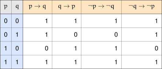
Notice that the values in the $p \to q$ column exactly match the values in the contrapositive column. This tells us that an implication is always logically equivalent to its contrapositive; in other words,
$$p \to q \Longleftrightarrow \neg q \to \neg p.$$Additionally, the values in the converse column exactly match those of the inverse column. This tells us that an implication’s converse is logically equivalent to its inverse, meaning
$$q \to p \Longleftrightarrow \neg p \to \neg q.$$Yet again, this is worth highlighting.
Since we’ve figured out that an implication is logically equivalent to its contrapositive, we could have deduced that the converse and inverse are logically equivalent just by noticing that the inverse is the contrapositive of the converse (and vice versa).
So far, we’ve studied what an implication means on its own, and how it relates to variations like its converse, inverse, and contrapositive. Now we turn to a special kind of implication — one that’s true no matter what truth values its hypothesis and conclusion happen to take on. These implications are especially useful, since knowing one holds lets us deduce its conclusion with total certainty the moment its hypothesis is satisfied.
We already know, from the Law of Material Implication, that $p \to q$ is logically equivalent to $\neg p \lor q$. Before moving on, it’s worth building some intuition for why that’s true, and seeing what it buys us.
Suppose we have $p \to q$ where
\[ \begin{array}{rl} p\text{: } &\text{Alyssa studies for her Chemistry exam.} \\ q\text{: } &\text{Alyssa gets an A on her Chemistry exam.} \end{array} \]What can we deduce if we know $\neg p$ is true (meaning $p$ is false)? In this scenario, Alyssa doesn’t study for her Chemistry exam. Does this mean she doesn’t get an A on her Chemistry exam?
Not necessarily. Remember, all we know is that if she studies, she’ll get an A — we weren’t told $\neg p \to \neg q$. Perhaps the exam is easy enough that Alyssa doesn’t feel the need to study. Perhaps the exam is difficult, but Alyssa is comfortable enough with the material to work out correct answers with a little thought. On the other hand, the exam could be extremely difficult for Alyssa, so maybe she doesn’t get an A. All we can conclude is that she didn’t study — we can’t determine whether we have $q$ or $\neg q$.
What if we know we have $p$ instead of $\neg p$? Since we know that if Alyssa studies, she’ll get an A, knowing that $p$ happened tells us that $q$ happened as well. (Note that since we’re asserting $p \to q$ is true, we can’t have $p \to \neg q$.)
Our conclusion hinges entirely on the truth value of $p$: if $\neg p$ happened, we don’t get any additional conclusions, but if $p$ happened, we immediately know $q$ happens too. This is exactly the behavior of the disjunction $\neg p \lor q$ — which is precisely why $p \to q \Longleftrightarrow \neg p \lor q$ in the first place.
Keeping this equivalence in mind makes negating an implication far less error-prone. As a reminder, from the Simplifying Logical Expressions section, we already worked out that
$$\neg (p \to q) \Longleftrightarrow p \land \neg q,$$which lines up with what we’d expect: an implication is false exactly when $p$ is true and $q$ is false.
It’s worth emphasizing why parentheses matter here. An expression such as $\neg p \to q$ is shorthand for $(\neg p) \to q$ — the negation $\neg$ is the most tightly-binding operation in an expression, so it only applies to $p$, not to the whole implication. This is a very different statement from $\neg (p \to q)$, as the truth table below makes clear.
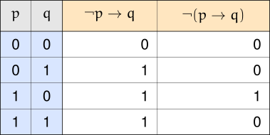
Any doubts about how an expression should be parsed can always be put to rest by adding parentheses of your own.
Consider two propositions $a$ and $b$, where
\[ \begin{array}{rl} a\text{: } &\text{Alvarez hauls up a red king crab pot.} \\ b\text{: } &\text{Alvarez has to report the catch to the harbormaster.} \end{array} \]Let’s compare two conjunctions built from these propositions and the implication $a \to b$: $a \land (a \to b)$, and $b \land (a \to b)$.
Suppose $a \land (a \to b)$ is true. Then $a$ is true — Alvarez hauls up a red king crab pot — and $a \to b$ is true as well. Since $a$ is true and $a \to b$ is true, we can deduce $b$ must be true too — Alvarez has to report the catch. So $a \land (a \to b)$ being true pins down both $a$ and $b$.
Now suppose $b \land (a \to b)$ is true instead. Then $b$ is true — Alvarez has to report the catch. But once $b$ is true, the implication $a \to b$ is automatically true too, no matter what $a$ happens to be — an implication with a true conclusion can never be false. So $b \land (a \to b)$ being true doesn’t actually tell us anything about $a$; it only ever tells us that $b$ is true.
The truth table below confirms that $[a \land (a \to b)] \to b$ is a tautology:
![The truth table for $a \\to b$, $a \\land (a \\to b)$, and $[a \\land (a \\to b)] \\to b$.](/books/foundational-mathematics/proof/logical-implications/02.svg)
Every row in the $[a \land (a \to b)] \to b$ column is a $1$, so $a \land (a \to b)$ always forces $b$ to be true.
Now compare that against the truth table for $[b \land (a \to b)] \to a$:
![The truth table for $a \\to b$, $b \\land (a \\to b)$, and $[b \\land (a \\to b)] \\to a$.](/books/foundational-mathematics/proof/logical-implications/03.svg)
Here, the $[b \land (a \to b)] \to a$ column has a single $0$, so this implication is not a tautology — $b \land (a \to b)$ being true doesn’t let us conclude $a$.
There’s a special name for these kinds of implications.
Suppose $a$ and $b$ are any arbitrary statements (primitive or compound) such that the implication $a \to b$ is always true — in other words, a tautology. We say that $a$ logically implies $b$, and we write
$$a \Longrightarrow b.$$If $a \to b$ is not a tautology, we write $a \not\Longrightarrow b$.
Based on the previous example, where we saw that $(a \land (a \to b)) \to b$ was a tautology, we can use this new notation and write
$$(a \land (a \to b)) \Longrightarrow b.$$Now that we’ve taken a closer look at the implication itself, let’s revisit quantified statements to see how the same ideas — logical implication, and the converse, inverse, and contrapositive — carry over to them.
Suppose we have some open statement $p(x)$ with some non-empty universe $\mathcal{U}$ (non-empty just means $\mathcal{U}$ contains at least one element, which we can refer to as $\alpha$).
What can we conclude if we know that the statement $\forall x\ [p(x)]$ is true — that is, we know $\forall x\ [p(x)] = 1$?
One thing we can conclude is that if $\alpha \in \mathcal{U}$ (meaning $\alpha$ is some element found within the universe $\mathcal{U}$), then $p(\alpha) = 1$. Since some value of $x$ exists that makes $p(x) = 1$, we can conclude that $\exists x\ [p(x)] = 1$.
Let our universe, denoted $N$, consist of the integers $1$ through $9$. Consider the open statement
\[ \begin{array}{rl} \ell(n)\text{: } &n^2 < 100 \end{array} \]defined on $N$. We know that $\forall n\ [\ell(n)]$ is true, because
\[ \begin{array}{lll} 1^2 = 1 < 100 & 4^2 = 16 < 100 & 7^2 = 49 < 100 \\ 2^2 = 4 < 100 & 5^2 = 25 < 100 & 8^2 = 64 < 100 \\ 3^2 = 9 < 100 & 6^2 = 36 < 100 & 9^2 = 81 < 100 \end{array} \]As such, we know that $\exists n\ [\ell(n)]$ is also true, since we know $1^2 = 1 < 100$, meaning there exists some value ($n = 1$) such that $\ell(n) = 1$.
Does this work the other way? That is, does knowing that $\exists x\ [p(x)]$ is true mean that $\forall x\ [p(x)]$ is true? Certainly not — knowing that some value exists that makes $p(x) = 1$ is not the same thing as knowing that every value of $x$ within $\mathcal{U}$ makes $p(x) = 1$.
Consider the universe, which we’ll denote $R$, consisting of all the real numbers. On that universe, consider the open statement
\[ \begin{array}{rl} r(x)\text{: } &1 - x^2 = 0. \end{array} \]We know that $\exists x\ [r(x)] = 1$. For example, $r(1) = 1$; we even have $r(-1) = 1$, for a total of two values that make $r(x)$ true.
However, notice that $1 - (2)^2 = -3$, so $r(2) = 0$. Since not every value of $x$ makes $r(x) = 1$, we have $\forall x\ [r(x)] = 0$.
This leads us to our first logical implication:
$$\forall x\ [p(x)] \Longrightarrow \exists x\ [p(x)].$$As a reminder, $\forall x\ [p(x)]$ is a single statement with a definite truth value — it’s not an open statement or a propositional function. The statement being expressed is that “every value of $x$ within $\mathcal{U}$ makes $p(x)$ true.” Likewise, $\exists x\ [p(x)]$ is also a single statement, which can be translated as “there exists at least one value of $x$ that makes $p(x)$ true.”
Another way to state this is to say that $\forall x\ [p(x)] \to \exists x\ [p(x)]$ is a tautology, where $\forall x\ [p(x)]$ is the hypothesis of the implication, and $\exists x\ [p(x)]$ is the conclusion.
Just like with ordinary statements, we can ask whether one open statement logically implies another.
Consider open statements $p(x)$ and $q(x)$ defined on some universe $\mathcal{U}$.
When $p(a) \to q(a) = 1$ for every value $a$ within $\mathcal{U}$ — in other words, when $p(a) \to q(a)$ is a tautology — we say $p(x)$ logically implies $q(x)$, and we write
$$\forall x\ [p(x) \Longrightarrow q(x)].$$Consider the universe of all planar quadrilaterals, along with the open statements
\[ \begin{array}{rl} s(q)\text{: } &\text{Quadrilateral } q \text{ is a square.} \\ r(q)\text{: } &\text{Quadrilateral } q \text{ is a rectangle.} \end{array} \]From classical geometry, we know that every square is a rectangle, but not every rectangle is a square. Thus, for every planar quadrilateral $q_0$,
$$s(q_0) \Longrightarrow r(q_0)$$but
$$r(q_0) \not\Longrightarrow s(q_0),$$and so $\forall q\ [s(q) \Longrightarrow r(q)]$.
Recall from the previous chapter that the existential quantifier distributes over disjunction, and the universal quantifier distributes over conjunction:
$$\exists x\ [p(x) \lor q(x)] \Longleftrightarrow \exists x\ [p(x)] \lor \exists x\ [q(x)],$$$$\forall x\ [p(x) \land q(x)] \Longleftrightarrow \forall x\ [p(x)] \land \forall x\ [q(x)].$$We also saw that the other pairing — the existential quantifier with conjunction, and the universal quantifier with disjunction — doesn’t distribute the same way. Now that we have the language of logical implication, we can pin down exactly what does survive in those two cases.
Suppose $\exists x\ [p(x) \land q(x)]$ is true. Then some value $a$ within $\mathcal{U}$ makes $p(a) \land q(a)$ true, which means $p(a)$ is true and $q(a)$ is true individually. Since $a$ makes $p(x)$ true, $\exists x\ [p(x)]$ is true; since $a$ also makes $q(x)$ true, $\exists x\ [q(x)]$ is true. So both $\exists x\ [p(x)]$ and $\exists x\ [q(x)]$ are true, meaning $\exists x\ [p(x)] \land \exists x\ [q(x)]$ is true as well. This holds no matter what $p(x)$ and $q(x)$ are, so
$$\exists x\ [p(x) \land q(x)] \Longrightarrow \bigl(\exists x\ [p(x)] \land \exists x\ [q(x)]\bigr).$$Consider the universe of all integers, along with the open statements
\[ \begin{array}{rl} p(x)\text{: } &x \text{ is even.} \\ q(x)\text{: } &x \text{ is a perfect square.} \end{array} \]Since $x = 4$ is both even and a perfect square, $\exists x\ [p(x) \land q(x)]$ is true. As expected, that same $x = 4$ also makes $p(x)$ true on its own and makes $q(x)$ true on its own, so $\exists x\ [p(x)] \land \exists x\ [q(x)]$ is true too — exactly what the implication guarantees.
By a similar argument, suppose $\forall x\ [p(x)] \lor \forall x\ [q(x)]$ is true. Then at least one of $\forall x\ [p(x)]$ or $\forall x\ [q(x)]$ is true. If $\forall x\ [p(x)]$ is true, then every value of $x$ within $\mathcal{U}$ makes $p(x)$ true, which certainly means every value of $x$ makes $p(x) \lor q(x)$ true as well — so $\forall x\ [p(x) \lor q(x)]$ is true. The same reasoning applies if instead $\forall x\ [q(x)]$ is the true one. Either way,
$$\bigl(\forall x\ [p(x)] \lor \forall x\ [q(x)]\bigr) \Longrightarrow \forall x\ [p(x) \lor q(x)].$$Consider the universe of all integers, along with the open statements
\[ \begin{array}{rl} p(x)\text{: } &x^2 \geq 0 \\ q(x)\text{: } &x \text{ is negative.} \end{array} \]Every integer satisfies $p(x)$, so $\forall x\ [p(x)]$ is true, meaning $\forall x\ [p(x)] \lor \forall x\ [q(x)]$ is true. As expected, every integer also satisfies $p(x) \lor q(x)$, since $p(x)$ alone is already true for every $x$ — so $\forall x\ [p(x) \lor q(x)]$ is true too.
Let $p(x)$ and $q(x)$ be any propositional functions defined on some universe $\mathcal{U}$.
\[ \begin{array}{lcl} \exists x\ [p(x) \land q(x)] & \Longrightarrow & \exists x\ [p(x)] \land \exists x\ [q(x)] \\ \forall x\ [p(x)] \lor \forall x\ [q(x)] & \Longrightarrow & \forall x\ [p(x) \lor q(x)] \end{array} \]Just like how the statement $p \to q$ has a converse, inverse, and contrapositive, so does the universally quantified statement $\forall x\ [p(x) \to q(x)]$.
Consider open statements $p(x)$ and $q(x)$ defined on some universe $\mathcal{U}$.
The converse of the statement $\forall x\ [p(x) \to q(x)]$ is
$$\forall x\ [q(x) \to p(x)].$$The inverse of the statement $\forall x\ [p(x) \to q(x)]$ is
$$\forall x\ [\neg p(x) \to \neg q(x)].$$The contrapositive of the statement $\forall x\ [p(x) \to q(x)]$ is
$$\forall x\ [\neg q(x) \to \neg p(x)].$$Just as an ordinary implication is logically equivalent to its contrapositive, a quantified implication is logically equivalent to its contrapositive. Furthermore, the converse and inverse of a quantified implication are logically equivalent to each other.
Consider the universe of all planar quadrilaterals, along with the open statements
\[ \begin{array}{rl} s(q)\text{: } &\text{Quadrilateral } q \text{ is a square.} \\ e(q)\text{: } &\text{Quadrilateral } q \text{ is equilateral.} \end{array} \]From classical geometry, we know that if a quadrilateral is a square, then it’s equilateral, so the statement $\forall q\ [s(q) \to e(q)]$ is a tautology. In other words, $\forall q\ [s(q) \Longrightarrow e(q)]$.
The contrapositive of the above statement is $\forall q\ [\neg e(q) \to \neg s(q)]$, which says that if a quadrilateral isn’t equilateral, then it isn’t a square. Since the original implication is a logical implication, so is the contrapositive, and so
$$\forall q\ [s(q) \to e(q)] \Longleftrightarrow \forall q\ [\neg e(q) \to \neg s(q)].$$Now let’s consider the converse, $\forall q\ [e(q) \to s(q)]$, which says that if a quadrilateral is equilateral, then it’s a square. This isn’t necessarily true — every rhombus is equilateral, but not every rhombus is a square. As such, $\forall q\ [e(q) \not\Longrightarrow s(q)]$.
The inverse can be written as $\forall q\ [\neg s(q) \to \neg e(q)]$, which says that if a quadrilateral isn’t a square, then it isn’t equilateral — but again, any non-square rhombus is equilateral. As such, $\forall q\ [\neg s(q) \not\Longrightarrow \neg e(q)]$.
Consider the universe of all real numbers, along with the open statements
\[ \begin{array}{rl} f(x)\text{: } &x^2 - 1 \geq 0 \\ \alpha(x)\text{: } &x \leq -1 \end{array} \]and the following quantified statements:
\[ \begin{array}{ll} \text{Statement:} &\forall x\ [f(x) \to \alpha(x)] \\ \text{Contrapositive:} &\forall x\ [\neg \alpha(x) \to \neg f(x)] \\ \text{Converse:} &\forall x\ [\alpha(x) \to f(x)] \\ \text{Inverse:} &\forall x\ [\neg f(x) \to \neg \alpha(x)] \end{array} \]Consider $x = 5$: $f(5) = 1$ and $\alpha(5) = 0$. Since $1 \to 0 = 0$, we have that $5$ is a counter-example, and so $\forall x\ [f(x) \to \alpha(x)] = 0$. Since $\forall x\ [f(x) \to \alpha(x)] \Longleftrightarrow \forall x\ [\neg \alpha(x) \to \neg f(x)]$, we also have $\forall x\ [\neg \alpha(x) \to \neg f(x)] = 0$.
We know the converse is true, since when $x \leq -1$, we have $x^2 \geq 1$, giving us $x^2 - 1 \geq 0$. Thus, $\forall x\ [\alpha(x) \to f(x)] = 1$, and since $\forall x\ [\alpha(x) \to f(x)] \Longleftrightarrow \forall x\ [\neg f(x) \to \neg \alpha(x)]$, we also have $\forall x\ [\neg f(x) \to \neg \alpha(x)] = 1$.
Consider the universe of all real numbers, along with the open statements from the previous example, together with a new one:
\[ \begin{array}{rl} f(x)\text{: } &x^2 - 1 \geq 0 \\ \alpha(x)\text{: } &x \leq -1 \\ \beta(x)\text{: } &x \geq 1 \end{array} \]Now consider the following quantified statements:
\[ \begin{array}{ll} \text{Statement:} &\forall x\ [f(x) \to (\alpha(x) \lor \beta(x))] \\ \text{Contrapositive:} &\forall x\ [\neg(\alpha(x) \lor \beta(x)) \to \neg f(x)] \\ \text{Converse:} &\forall x\ [(\alpha(x) \lor \beta(x)) \to f(x)] \\ \text{Inverse:} &\forall x\ [\neg f(x) \to \neg(\alpha(x) \lor \beta(x))] \end{array} \]The converse and inverse both remain true, since all we did was introduce a disjunction. But now the original statement is also true:
$$\forall x\ [f(x) \to (\alpha(x) \lor \beta(x))] \Longleftrightarrow \forall x\ [\neg(\alpha(x) \lor \beta(x)) \to \neg f(x)] = 1.$$Furthermore, since we know both the original statement and the converse are true, we can write
$$\forall x\ [f(x) \leftrightarrow (\alpha(x) \lor \beta(x))] = 1,$$or equivalently, $\forall x\ [f(x) \Longleftrightarrow (\alpha(x) \lor \beta(x))]$.
Reconsider the earlier example where we considered the universe of all planar quadrilaterals with
\[ \begin{array}{rl} s(q)\text{: } &\text{Quadrilateral } q \text{ is a square.} \\ e(q)\text{: } &\text{Quadrilateral } q \text{ is equilateral.} \end{array} \]From classical geometry, we know that some equilateral quadrilaterals aren’t squares, so $\forall q\ [e(q) \to s(q)] = 0$. Thus, $\neg \forall q\ [e(q) \to s(q)] = 1$.
Using the negation equivalencies from the previous section, we have $\exists q\ [\neg(e(q) \to s(q))] = 1$. We can negate the inner implication with the following steps:
\[ \begin{array}{lll} & \boldsymbol{\exists q\ [\neg(e(q) \to s(q))]} & \textbf{Reason} \\ \Longleftrightarrow & \exists q\ [\neg(\neg e(q) \lor s(q))] & \text{Law of Material Implication} \\ \Longleftrightarrow & \exists q\ [\neg \neg e(q) \land \neg s(q)] & \text{DeMorgan's Law} \\ \Longleftrightarrow & \exists q\ [e(q) \land \neg s(q)] & \text{Law of Double Negation} \end{array} \]Thus, we know $\exists q\ [e(q) \land \neg s(q)] = 1$, meaning there exists some planar quadrilateral that’s equilateral, but not a square. One such example is a rhombus with opposite angle measures of $60°$ and $120°$.
The heart of mathematics is not mere computation, but the act of taking a combination of known facts and combining them in some way to arrive at new conclusions. Think back to when you learned the Pythagorean Theorem or the Quadratic Formula. It’s certainly true that these tools help you compute things — the hypotenuse of a right triangle, or the roots of a quadratic function — but that’s a computational activity.
Without the Pythagorean Theorem or the Quadratic Formula, how would we go about computing those quantities in the first place? There may be other methods available, but those two tools in particular are extremely helpful — and the reason they exist is that someone took what was already known about right triangles and quadratic expressions, and arrived at the now-famous results. The difference between doing mathematics and computing is a little like this: mathematics is knowing that for all right triangles, where the legs have lengths $a$ and $b$, and the hypotenuse has length $c$, we have
$$a^2 + b^2 = c^2;$$computation is figuring out that a right triangle with leg lengths $5$ and $12$ has a hypotenuse of length $13$ using the Pythagorean Theorem.
In order to know anything in mathematics, we start with what’s currently known, and extrapolate from that prior knowledge. We call this providing an argument, or a proof. In this section, we examine the basic structure of such an argument.
Let’s elaborate on the idea of using existing knowledge. We essentially take a collection of known facts together, and their combination provides some new fact:
\[ \begin{array}{ll} \text{IF} & \text{known fact \#1} \\ \text{AND} & \text{known fact \#2} \\ \text{AND} & \text{known fact \#3} \\ & \vdots \\ \text{AND} & \text{known fact \#}n \\ \text{THEN} & \text{new fact.} \end{array} \]Notice that we combine several facts using the word “and.” All the facts are supposed to come together in order to create the new fact — if any fact could be left out, then it wasn’t needed. This is the same situation we had with the conjunction $\land$: every proposition attached to a conjunction has to be true in order for the conjunction itself to be true.
Let’s rewrite the representation above using mathematical notation, where $p_1$ represents known fact #1 (a fact is just another term for a proposition), $p_2$ represents known fact #2, and so on through $p_n$ for known fact #$n$, with the letter $c$ denoting the new fact:
$$(p_1 \land p_2 \land p_3 \land \dots \land p_n) \to c.$$Consider a collection of $n+1$ propositions $p_1, p_2, p_3, \dots, p_n, c$. An implication of the form
$$(p_1 \land p_2 \land p_3 \land \dots \land p_n) \to c$$is called an argument. The propositions $p_1, p_2, p_3, \dots, p_n$ within the repeated conjunction are called the premises of the argument. The proposition $c$ is called the conclusion of the argument.
Notice that this definition doesn’t require the premises to be primitive propositions — each premise can be primitive, or it can be some long, complicated compound proposition. What matters is that we combine all of the premises into a conjunction.
Let $a$, $b$, $c$ represent the following propositions:
\[ \begin{array}{rl} a\text{: } &\text{The vault door is locked overnight.} \\ b\text{: } &\text{A thief breaks into the vault.} \\ c\text{: } &\text{The morning audit turns up clean.} \end{array} \]Now consider an argument with the following premises:
\[ \begin{array}{rl} p_1\text{: } &a \to c \\ p_2\text{: } &\neg b \to a \\ p_3\text{: } &\neg c \end{array} \]The argument we want to examine is $(p_1 \land p_2 \land p_3) \to b$.
We know that an implication is only false when the hypothesis is true and the conclusion is false. Working through a truth table for all three atomic propositions confirms that, in every row where $p_1 \land p_2 \land p_3$ is true, the conclusion $b$ is true as well — meaning the overall implication $(p_1 \land p_2 \land p_3) \to b$ has $1$s all the way down its column, and is a tautology.
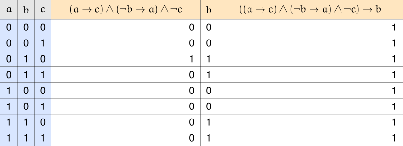
As such, we can write
$$(p_1 \land p_2 \land p_3) \Longrightarrow b.$$So, the argument is a logical implication. Therefore, if
\[ \begin{array}{l} \text{The vault door is locked overnight, then the morning audit turns} \\ \text{up clean;} \\[0.75em] \text{If no thief breaks into the vault, then the vault door is locked} \\ \text{overnight; and} \\[0.75em] \text{The morning audit does not turn up clean} \end{array} \]are all true propositions, then a thief likely broke into the vault somehow.
The previous example demonstrates something important about arguments: an argument asserts that, when all premises are true, the conclusion is also true. If there’s a scenario where all premises are true but the conclusion isn’t, then that argument doesn’t accurately reflect when the conclusion is true.
In order for an argument to accurately reflect when its conclusion is true, the conclusion must be true whenever the premises are true — otherwise, the argument is simply wrong.
On the other hand, we don’t care what happens when any of the premises are false. An argument only tells us that if all premises are true, then so is the conclusion — it’s irrelevant when any premise is false.
Consider an argument of the form $(p_1 \land p_2 \land p_3 \land \dots \land p_n) \to c$. If the implication is a tautology — that is, if it’s a logical implication with
$$(p_1 \land p_2 \land p_3 \land \dots \land p_n) \Longrightarrow c,$$then we call the argument a valid argument.
Mathematics is all about developing valid arguments, because these arguments form the base of the knowledge we have. Arguments give us a way to come up with new and efficient ways to perform computations, make classifications, or establish any other kind of equivalency.
Consider three propositions $x$, $y$, $z$ — none of which have to be primitive, they just each denote some proposition, whether simple, complex, or anywhere in between.
Now consider the following argument:
$$(p_1 \land p_2) \to c$$where
\[ \begin{array}{rl} p_1\text{: } &x \to y \\ p_2\text{: } &y \to z \\ c\text{: } &x \to z \end{array} \]Filling out a truth table for $x$, $y$, $z$ and each of these propositions in turn confirms that the column for $[(x \to y) \land (y \to z)] \to (x \to z)$ is entirely $1$s.
![The truth table for $x \\to y$, $y \\to z$, $(x \\to y) \\land (y \\to z)$, $x \\to z$, and $[(x \\to y) \\land (y \\to z)] \\to (x \\to z)$.](/books/foundational-mathematics/proof/arguments/02.svg)
As such, the argument
$$[(x \to y) \land (y \to z)] \to (x \to z)$$is valid. Therefore, if we ever run into a situation where we know that $x \to y$ and that $y \to z$, then we know that $x \to z$ as well, where $x$, $y$, and $z$ represent arbitrary propositions.
We’ve already seen that, with ever-larger numbers of component propositions, a truth table requires more and more rows to complete — and that logical equivalencies let us simplify compound propositions without needing a truth table at all.
We can bypass truth tables when determining whether an argument is valid too. Instead of logical equivalencies, though, we use logical implications. In this section, we collect a list of commonly occurring logical implications, and see how to use them strategically. We’ll still verify each one with a truth table — the point here is just to build up a list of implications we can use later.
We introduce the first logical implication with an example.
Suppose a mechanic is servicing a car with a rough idle, and knows from experience that replacing a worn timing belt often fixes the issue. Consider the propositions
\[ \begin{array}{rl} p\text{: } &\text{The mechanic replaces the car's timing belt.} \\ q\text{: } &\text{The car's engine runs smoothly.} \end{array} \]We know that if the mechanic replaces the timing belt, then the engine runs smoothly — that is, $p \to q = 1$. This alone doesn’t tell us whether the engine runs smoothly, because if $p = 0$, the implication is still true regardless of whether $q = 0$ or $q = 1$.
However, suppose we also know that $p = 1$ — the mechanic did replace the timing belt. Now we do know that the engine runs smoothly, because both $p = 1$ and $p \to q = 1$. The only way for both of these propositions to be true is for $q = 1$.
We can verify this more formally with a truth table (representing $p$ as premise $p_1$, the proposition $p \to q$ as premise $p_2$, and the conclusion $q$ using the letter $c$): the column for $[p \land (p \to q)] \to q$ is entirely $1$s, so
$$[p \land (p \to q)] \Longrightarrow q.$$In other words, whenever we know $p$ is true, and $p \to q$ is true, then $q$ is true as well. As such, the argument $[p \land (p \to q)] \to q$ is valid. It’s common to write this kind of argument out in tabular form: we list all the premises in a single column, add a horizontal line, and write the conclusion below it, with a $\therefore$ symbol (read “therefore,” or “thus”) to its left:
\[ \begin{array}{l} p \\ p \to q \\ \hline \therefore q \end{array} \]Also note that because $\land$ is commutative, we could just as well present this argument with its premises in the other order:
\[ \begin{array}{l} p \to q \\ p \\ \hline \therefore q \end{array} \]This kind of argument is commonly referred to as Modus Ponens.
There’s another kind of valid argument closely related to Modus Ponens. Again, we demonstrate it with an example first.
Returning to the mechanic and the timing belt, we know $p \to q = 1$. This means there are only three possible combinations of truth values for $p$ and $q$: $p = 0, q = 0$; $p = 0, q = 1$; and $p = 1, q = 1$.
If $q = 1$, we don’t know whether $p = 0$ or $p = 1$. But if we happened to know that $q = 0$, we’d definitely know that $p = 0$. In other words, it seems as if we have
$$[(p \to q) \land \neg q] \to \neg p.$$In the context of this example, this means that if we knew “If the mechanic replaces the timing belt, then the engine runs smoothly” and “The engine does not run smoothly” were both true, we’d also know “The mechanic did not replace the timing belt” was true.
A truth table confirms that $[(p \to q) \land \neg q] \to \neg p$ is indeed a tautology, so
$$[(p \to q) \land \neg q] \Longrightarrow \neg p.$$The argument
\[ \begin{array}{l} \neg q \\ p \to q \\ \hline \therefore \neg p \end{array} \]is valid, as is the same argument with its premises swapped. This argument is commonly referred to as Modus Tollens. Both Modus Ponens and Modus Tollens have $p \to q$ as a premise — in some sense, Modus Tollens is the “contrapositive” of Modus Ponens.
The argument
\[ \begin{array}{l} p \to q \\ q \to r \\ \hline \therefore p \to r \end{array} \]is valid — we already confirmed this in the previous section, where we showed $[(x \to y) \land (y \to z)] \to (x \to z)$ is a tautology. This argument is commonly referred to as the Law of the Syllogism.
Because $\land$ is commutative, the premises of any argument can be swapped and the argument remains valid — a fact we won’t keep explicitly mentioning, though it will be used implicitly throughout our work.
Naturally, we can chain more and more propositions together at the end of each premise’s implication. Here’s an example involving five propositions:
\[ \begin{array}{l} j \to a \\ a \to c \\ c \to o \\ o \to b \\ \hline \therefore j \to b \end{array} \]Not all of the arguments at our disposal are profound — some may seem quite obvious. For instance, suppose we know proposition $p$ is true, and proposition $q$ is true. Since they’re both true, we also know their conjunction $p \land q$ is true. The argument
\[ \begin{array}{l} p \\ q \\ \hline \therefore p \land q \end{array} \]is valid, and is called the Rule of Conjunction. Why care about an argument this simple? Because as we develop more sophisticated arguments, propositions $p$ and $q$ may come up — either as premises, or as results derived from other premises. When this happens, $p$ and $q$ can be combined into a conjunction, and that conjunction can be used to further develop the argument, as we’ll see used strategically in the next section.
Suppose a car won’t start, and a mechanic determines that the problem must be either a dead battery or a faulty starter. Define
\[ \begin{array}{rl} M\text{: } &\text{The car's battery is dead.} \\ L\text{: } &\text{The car's starter is faulty.} \end{array} \]Since the mechanic is confident it’s one or the other, $M \lor L = 1$. Right now, we don’t know which it is — but suppose the mechanic also tests the starter and finds it works fine, meaning $\neg L = 1$. Since $M \lor L = 1$ and $L = 0$, we’d have to have $M = 1$, meaning the battery is dead. We can represent this as the argument $[(M \lor L) \land \neg L] \to M$.
As this example demonstrates, if we know at least one of two propositions $p$ and $q$ is true, but that one of them (say $q$) is false, then the other must be true — otherwise the disjunction would have been false. The argument
\[ \begin{array}{l} p \lor q \\ \neg q \\ \hline \therefore p \end{array} \]is valid, and is called the Rule of Disjunctive Syllogism. A truth table readily confirms this.
Suppose we’re given some proposition $p$, and want to determine whether $p = 0$ or $p = 1$. One thing we could try is to assume $p = 0$ (meaning $\neg p = 1$). If assuming $p = 0$ yields a contradiction $F_0$, then surely $p \neq 0$, since true statements should never yield contradictions — hence we must have $p = 1$. The argument
\[ \begin{array}{l} \neg p \to F_0 \\ \hline \therefore p \end{array} \]is valid, and is called the Rule of Contradiction. Since there’s only one premise, $\neg p \to F_0$ (a proposition that’s just $\neg p \to 0$, replacing the general contradiction $F_0$ with its truth value), there’s no conjunction operator present. A truth table confirms the argument $(\neg p \to F_0) \to p$ is valid.
We’ve presented five different kinds of arguments so far. These arguments are commonly referred to as rules of inference, because they let us infer, or deduce, a conclusion given a list of premises. There are many more such rules; we present a sample of them below.
| Modus Ponens (Rule of Detachment) | $\begin{array}{l} p \\ p \to q \\ \hline \therefore q \end{array}$ | $[p \land (p \to q)] \Longrightarrow q$ |
| Modus Tollens | $\begin{array}{l} p \to q \\ \neg q \\ \hline \therefore \neg p \end{array}$ | $[(p \to q) \land \neg q] \Longrightarrow \neg p$ |
| Law of the Syllogism | $\begin{array}{l} p \to q \\ q \to r \\ \hline \therefore p \to r \end{array}$ | $[(p \to q) \land (q \to r)] \Longrightarrow (p \to r)$ |
| Rule of Conjunction | $\begin{array}{l} p \\ q \\ \hline \therefore p \land q \end{array}$ | $(p \land q) \Longrightarrow (p \land q)$ |
| Rule of Disjunctive Syllogism | $\begin{array}{l} p \lor q \\ \neg q \\ \hline \therefore p \end{array}$ | $[(p \lor q) \land \neg q] \Longrightarrow p$ |
| Rule of Contradiction | $\begin{array}{l} \neg p \to F_0 \\ \hline \therefore p \end{array}$ | $(\neg p \to F_0) \Longrightarrow p$ |
| Rule of Conjunctive Simplification | $\begin{array}{l} p \land q \\ \hline \therefore p \end{array}$ | $(p \land q) \Longrightarrow p$ |
| Rule of Disjunctive Amplification | $\begin{array}{l} p \\ \hline \therefore p \lor q \end{array}$ | $p \Longrightarrow (p \lor q)$ |
| Rule of Conditional Proof | $\begin{array}{l} p \land q \\ p \to (q \to r) \\ \hline \therefore r \end{array}$ | $[(p \land q) \land (p \to (q \to r))] \Longrightarrow r$ |
| Rule of Proof by Cases | $\begin{array}{l} p \to r \\ q \to r \\ \hline \therefore (p \lor q) \to r \end{array}$ | $[(p \to r) \land (q \to r)] \Longrightarrow [(p \lor q) \to r]$ |
| Rule of the Constructive Dilemma | $\begin{array}{l} p \to q \\ r \to s \\ p \lor r \\ \hline \therefore q \lor s \end{array}$ | $[(p \to q) \land (r \to s) \land (p \lor r)] \Longrightarrow (q \lor s)$ |
| Rule of the Destructive Dilemma | $\begin{array}{l} p \to q \\ r \to s \\ \neg q \lor \neg s \\ \hline \therefore \neg p \lor \neg r \end{array}$ | $[(p \to q) \land (r \to s) \land (\neg q \lor \neg s)] \Longrightarrow (\neg p \lor \neg r)$ |
Before seeing how these rules of inference can be used, it’s worth taking a step back to see what we’ve accomplished — but perhaps more importantly, what we have not accomplished.
Notice that each rule of inference above is a logical implication — demonstrated by the fact that we used the single arrow $\Longrightarrow$, rather than the double arrow $\Longleftrightarrow$. While some of the arguments above may happen to contain logical equivalencies (such as the Rule of Conjunction), most of these are not logical equivalencies.
For instance, examining the Law of the Syllogism, we have
$$[(p \to q) \land (q \to r)] \Longrightarrow (p \to r).$$However, note that when $p = r = 0$ and $q = 1$, we have $(p \to q) = 1$, $(q \to r) = 0$, and $(p \to r) = 1$, but $(p \to q) \land (q \to r) = 1 \land 0 = 0$. Hence,
$$[(p \to q) \land (q \to r)] \not\Longleftrightarrow (p \to r).$$As such, we have not shown that the expression $(p \to q) \land (q \to r)$ can be replaced with the simpler expression $p \to r$. This is a subtle difference, but an important one.
We’ll see in the next section that both logical equivalencies and logical implications can be used to develop arguments — but logical implications won’t be helpful when trying to simplify complicated logical expressions.
In the previous section, we collected a large sample of commonly occurring logical implications. We briefly touched on why we’d want such a list — to determine whether a given argument is valid. In addition to determining validity, we can also use the rules of inference to make valid deductions from a given list of premises.
In this section, we work through several examples of both use cases.
Suppose we’re presented with some argument: a list of premises, and a desired conclusion. We can determine if the argument is valid by appealing to the rules of inference.
Because you love live rock music, you decide to purchase front-row tickets for an upcoming rock concert. The tickets are expensive, so you’ll need to save up money working a summer job to purchase them. The problem is that everybody wants front-row seats, so they may be sold out by the time you have enough money.
Consider the propositions
\[ \begin{array}{rl} a\text{: } &\text{You save up enough money to purchase front-row seats.} \\ b\text{: } &\text{There are no more front-row seats available.} \\ c\text{: } &\text{You sit front row at the rock concert.} \end{array} \]and the argument
\[ \begin{array}{l} \neg b \\ \neg b \to a \\ a \to c \\ \hline \therefore c \end{array} \]To determine whether this argument is valid, notice that because we have both $\neg b$ and $\neg b \to a$, we must have $a$ by Modus Ponens. Now, because we have both $a$ and $a \to c$, we also have $c$ by Modus Ponens.
We just reached the desired conclusion $c$ by appealing to Modus Ponens twice, meaning the argument is valid. So, if there are front-row seats available, you’ll be able to save up enough money to sit front row at the rock concert. Awesome!
It seems a bit cumbersome to write out our logic in paragraphs like this. Just like we did when showing two compound propositions were logically equivalent, we can write out a sequence of steps in tabular form.
Luckily for us, another rock concert is happening, which means we need to start saving even more money, hoping front-row seats are still available. Reconsider the argument from the previous example. We can write out the sequence of steps we took there in tabular form:
\[ \begin{array}{lll} \textbf{Step} & \textbf{Proposition} & \textbf{Reason} \\ (1) & \neg b & \text{Premise} \\ (2) & \neg b \to a & \text{Premise} \\ (3) & a & \text{Modus Ponens on Steps (1) and (2)} \\ (4) & a \to c & \text{Premise} \\ (5) & \therefore c & \text{Modus Ponens on Steps (3) and (4)} \end{array} \]Just like before, we reached conclusion $c$ using the rules of inference. We’ll use this tabular form of validating an argument from here on out.
There are many rules of inference, so we may be able to validate a given argument in multiple different ways.
Let’s reconsider the argument once more. Instead of using Modus Ponens twice, we could look at the big list of inference rules from the previous section again. One rule that stands out is the Law of the Syllogism, since we have two implications as premises:
\[ \begin{array}{lll} \textbf{Step} & \textbf{Proposition} & \textbf{Reason} \\ (1) & \neg b \to a & \text{Premise} \\ (2) & a \to c & \text{Premise} \\ (3) & \neg b \to c & \text{Law of the Syllogism on Steps (1) and (2)} \\ (4) & \neg b & \text{Premise} \\ (5) & \therefore c & \text{Modus Ponens on Steps (3) and (4)} \end{array} \]Of course, we arrive yet again at the desired conclusion $c$.
Going forward, when we write out these tabular arguments, we’ll omit the word “Steps,” and just write out which numbered step is being used in a rule of inference — this will save us a bit of writing. It’s also worth pointing out that since some propositions are given as premises, they require no justification beyond noting they’re premises of the argument.
Some arguments require multiple rules of inference to determine validity.
Consider the following argument, with propositions $s$, $t$, $x$, $y$, and $z$:
\[ \begin{array}{l} x \\ x \to y \\ s \lor t \\ t \to \neg y \\ \hline \therefore s \lor z \end{array} \]We could take the following steps to validate this argument:
\[ \begin{array}{lll} \textbf{Step} & \textbf{Proposition} & \textbf{Reason} \\ (1) & x & \text{Premise} \\ (2) & x \to y & \text{Premise} \\ (3) & y & \text{Modus Ponens on (1) and (2)} \\ (4) & t \to \neg y & \text{Premise} \\ (5) & y \to \neg t & \text{Contrapositive of (4): } (t \to \neg y) \Longleftrightarrow (y \to \neg t) \\ (6) & \neg t & \text{Modus Ponens on (3) and (5)} \\ (7) & s \lor t & \text{Premise} \\ (8) & s & \text{Rule of Disjunctive Syllogism on (6) and (7)} \\ (9) & \therefore s \lor z & \text{Rule of Disjunctive Amplification on (8)} \end{array} \]So, we arrive at the desired conclusion $s \lor z$, using a wide variety of rules of inference.
In the previous example, step (5) made use of a logical equivalency between contrapositives. As we work through an argument, we can introduce logically equivalent propositions whenever we want — so we should make use of this as much as possible.
For arbitrary propositions $a$, $b$, $c$, $d$, $e$, and $f$, consider the argument
\[ \begin{array}{l} a \to e \\ e \to (b \land c) \\ \neg c \lor (f \lor \neg d) \\ d \land a \\ \hline \therefore f \end{array} \]This one may require a lot of work, so let’s get started:
\[ \begin{array}{lll} \textbf{Step} & \textbf{Proposition} & \textbf{Reason} \\ (1) & a \to e & \text{Premise} \\ (2) & e \to (b \land c) & \text{Premise} \\ (3) & a \to (b \land c) & \text{Law of the Syllogism on (1) and (2)} \\ (4) & d \land a & \text{Premise} \\ (5) & a & \text{Conjunctive Simplification on (4)} \\ (6) & b \land c & \text{Modus Ponens on (3) and (5)} \\ (7) & c & \text{Conjunctive Simplification on (6)} \\ (8) & \neg c \lor (f \lor \neg d) & \text{Premise} \\ (9) & f \lor \neg d & \text{Disjunctive Syllogism on (7) and (8)} \\ (10) & d & \text{Conjunctive Simplification on (4)} \\ (11) & \therefore f & \text{Disjunctive Syllogism on (9) and (10)} \end{array} \]When determining whether an argument is valid, we’re given a list of premises and a conclusion, and we write out our justifications in tabular form, with the conclusion as the table’s last entry. Theoretically, we could do the same thing even without being given a conclusion — we just wouldn’t have a “goal” to reach. We could apply whatever rule of inference seems appropriate to the given premises, and to any previous conclusions reached from them.
Consider the propositions
\[ \begin{array}{rl} c\text{: } &\text{I am clever.} \\ \ell\text{: } &\text{I am lucky.} \\ w\text{: } &\text{I win the lottery.} \end{array} \]and the premises $c \lor \ell$, $\neg \ell$, and $\ell \to w$. We’re not given a conclusion, but can we make any inference from these premises?
One conclusion we could easily reach is to use the Rule of Disjunctive Syllogism on the first two premises, giving us conclusion $c$. As such, we know the argument $[(c \lor \ell) \land \neg \ell \land (\ell \to w)] \to c$ is valid.
Note that once you use a rule of inference on a given list of premises, you’re making a valid argument — every intermediate step in the previous section’s longer example produced a valid argument, since each was constructed by means of a rule of inference.
Consider the premises
\[ \begin{array}{l} \text{If the band can't perform their concert, or their t-shirts aren't} \\ \text{available for purchase at the concert, then the after-party will be} \\ \text{cancelled, and you will not purchase front-row seats. If the} \\ \text{after-party is cancelled, then ticket sales will have to be issued} \\ \text{refunds. No refunds were issued.} \end{array} \]We pick out the propositions
\[ \begin{array}{rl} a\text{: } &\text{The band can perform their concert.} \\ t\text{: } &\text{The band's t-shirts are available for purchase.} \\ p\text{: } &\text{The after-party was cancelled.} \\ y\text{: } &\text{You do not buy front-row seats.} \\ r\text{: } &\text{Ticket sales are issued refunds.} \end{array} \]giving us the premises $(\neg a \lor \neg t) \to (p \land y)$, $p \to r$, and $\neg r$. Let’s see what deductions we can make:
\[ \begin{array}{lll} \textbf{Step} & \textbf{Proposition} & \textbf{Reason} \\ (1) & p \to r & \text{Premise} \\ (2) & \neg r & \text{Premise} \\ (3) & \neg p & \text{Modus Tollens on (1) and (2)} \\ (4) & \neg p \lor \neg y & \text{Disjunctive Amplification on (3)} \\ (5) & \neg (p \land y) & \text{DeMorgan's Law on (4)} \\ (6) & (\neg a \lor \neg t) \to (p \land y) & \text{Premise} \\ (7) & \neg (\neg a \lor \neg t) & \text{Modus Tollens on (5) and (6)} \\ (8) & \neg \neg a \land \neg \neg t & \text{DeMorgan's Law on (7)} \\ (9) & a \land t & \text{Law of Double Negation on (8)} \\ (10) & a & \text{Conjunctive Simplification on (9)} \\ (11) & t & \text{Conjunctive Simplification on (9)} \end{array} \]Notice that one of our conclusions was $a$, in step (10). As such, we know that $[((\neg a \lor \neg t) \to (p \land y)) \land (p \to r) \land \neg r] \to a$ is a valid argument — with the given premises, we could deduce that the band performed their concert!
We didn’t stop at that one conclusion, though. Step (11) left us with conclusion $t$, meaning we could also deduce that the band’s t-shirts were available for purchase. Yet another inference we made was $\neg p$, in step (3), meaning the after-party was not cancelled!
Any of the intermediate propositions that weren’t premises are valid inferences from the given premises.
One more strategy we could use is a truth table, to see what combinations of truth values for the propositions yield true premises.
Consider the propositions
\[ \begin{array}{rl} s\text{: } &\text{Johnny had to go to summer school.} \\ j\text{: } &\text{Johnny could work a summer job.} \\ a\text{: } &\text{Johnny could purchase front-row seats at the rock concert.} \end{array} \]and the premises $s$, $s \to \neg j$, and $\neg j \to \neg a$. Constructing a truth table and checking which rows make all three premises true reveals only one combination: $s = 1$, $j = 0$, $a = 0$.
So, we need some combination of these three propositions that yields $1$ under that assignment. One such example is $\neg j$, meaning $[s \land (s \to \neg j) \land (\neg j \to \neg a)] \to \neg j$ is a valid argument. We also have $\neg a = 1$, so $[s \land (s \to \neg j) \land (\neg j \to \neg a)] \to \neg a$ is valid too.
Since $j = 0$ and $\neg a = 1$, we have $j \land \neg a = 0$, meaning $\neg (j \land \neg a) = 1$, and so $\neg j \lor a = 1$ as well. As such, the argument $[s \land (s \to \neg j) \land (\neg j \to \neg a)] \to (\neg j \lor a)$ is also valid.
It’s good practice to try and come up with a sequence of inference rules to reach these kinds of conclusions without going through a truth table.
Fundamentally, an argument is nothing more than a logical implication — a hypothesis (a conjunction of multiple premises) and a conclusion.
We’ve already seen that it’s possible to construct logically equivalent propositions using the laws of logic. Since an argument is fundamentally a proposition based on an implication, it should be possible to construct a different argument that’s logically equivalent to a given one. In some cases, this new, equivalent argument may be easier to verify than the original — which is exactly why it’s worth investing time in constructing logically equivalent arguments in the first place.
The general structure of an argument is
\[ \begin{array}{l} p_1 \\ p_2 \\ \vdots \\ p_n \\ \hline \therefore c \end{array} \]meaning we’re only considering cases where each premise $p_1$ through $p_n$ is true.
If we take the propositional form of this argument with just one premise, we get $p_1 \to c$. We’d need $c = 1$ for this implication to be true — but this is logically equivalent to $\neg p_1 \lor c$. We can extend this a bit further:
\[ \begin{array}{lll} & \boldsymbol{p_1 \to c} & \textbf{Reason} \\ \Longleftrightarrow & \neg p_1 \lor c & \text{Law of Material Implication} \\ \Longleftrightarrow & \neg (p_1 \land \neg c) & \text{DeMorgan's Law} \end{array} \]So, if $p_1 \to c$ is a valid argument, then $\neg (p_1 \land \neg c)$ is a true proposition. This means it would be impossible to have both $p_1 = 1$ and $c = 0$ — that is, both $p_1 = 1$ and $\neg c = 1$ — since that would be a contradiction. In other words, we get the argument $(p_1 \land \neg c) \to F_0$.
This is where this proof strategy gets its name: for a valid argument, assuming the negation of the desired conclusion produces a contradiction. Since the negation of the conclusion must therefore be false, the conclusion itself must be true.
A truth table confirms that $(p_1 \to c)$ and $[(p_1 \land \neg c) \to F_0]$ are logically equivalent — meaning the arguments themselves are equivalent, since arguments are just implications. So, establishing that one of these is valid means the other is valid too.
Frank is a farmer who loves being outdoors and working on his gardens. He grows two kinds of plants: sunflowers and wheat, though he can’t plant both in his garden at once, as the two kinds of plants may interfere with each other’s growth. Furthermore, if he grows wheat, he’ll be able to make his own bread.
Consider the propositions
\[ \begin{array}{rl} s\text{: } &\text{Frank plants sunflowers in his garden.} \\ w\text{: } &\text{Frank plants wheat in his garden.} \\ b\text{: } &\text{Frank bakes bread using the wheat he grew in his garden.} \end{array} \]We can express this situation as the argument
\[ \begin{array}{l} \neg s \leftrightarrow w \\ w \to b \\ \neg b \\ \hline \therefore s \end{array} \]In order to establish this argument’s validity, we could instead consider whether the equivalent argument
\[ \begin{array}{l} \neg s \leftrightarrow w \\ w \to b \\ \neg b \\ \neg s \\ \hline \therefore F_0 \end{array} \]is valid. To do so, we use the rules of inference and the laws of logic:
\[ \begin{array}{lll} \textbf{Step} & \textbf{Proposition} & \textbf{Reason} \\ (1) & \neg s \leftrightarrow w & \text{Premise} \\ (2) & (\neg s \to w) \land (w \to \neg s) & (a \leftrightarrow b) \Longleftrightarrow [(a \to b) \land (b \to a)] \\ (3) & \neg s \to w & \text{Conjunctive Simplification on (2)} \\ (4) & w \to b & \text{Premise} \\ (5) & \neg s \to b & \text{Law of the Syllogism on (3) and (4)} \\ (6) & \neg s & \text{Premise} \\ (7) & b & \text{Modus Ponens on (5) and (6)} \\ (8) & \neg b & \text{Premise} \\ (9) & b \land \neg b & \text{Rule of Conjunction on (7) and (8)} \\ (10) & \therefore F_0 & (b \land \neg b) \Longleftrightarrow F_0 \end{array} \]So, using the rules of inference, we’ve determined this equivalent argument is valid — meaning the original argument is valid too.
Therefore, if we know
\[ \begin{align*} &\text{Frank plants wheat if and only if he does not plant sunflowers.} \\ &\text{If Frank plants wheat, then Frank will make bread using wheat} \\ &\text{he grew in his garden.} \\ &\text{Frank does not make bread using wheat he grew in his garden.} \end{align*} \]are all true propositions, then we know Frank planted sunflowers in his garden.
Suppose we knew the argument
\[ \begin{array}{l} p \\ \hline \therefore q \to r \end{array} \]was valid. Since $p = 1$, we know $q \to r = 1$. But now suppose we also knew $q = 1$: since $q \to r = 1$ and $q = 1$, we’d have $r = 1$ as well. Notice that since $p = 1$ and $q = 1$, we have $p \land q = 1$. Writing this out as a proposition, we get $p \to (q \to r)$ — and since having both $p$ and $q$ necessarily gives us $r$, this becomes the argument $(p \land q) \to r$.
This suggests that the argument $p \to (q \to r)$ is logically equivalent to the argument $(p \land q) \to r$. A truth table confirms this suspicion: the biconditional $[p \to (q \to r)] \leftrightarrow [(p \land q) \to r]$ is a tautology, meaning we have a logical equivalency between the two arguments. Just as before, establishing the validity of one automatically establishes the validity of the other.
Frank has been thinking about using the wheat he grows to open a bakery where he sells fresh bread. Of course he’ll need a building to serve as his store, and he’ll need to make sure his tractor is working so he can actually farm his crops. Consider the propositions
\[ \begin{array}{rl} t\text{: } &\text{Frank fixes his tractor.} \\ s\text{: } &\text{Frank grows sunflowers in his garden.} \\ w\text{: } &\text{Frank grows wheat in his garden.} \\ b\text{: } &\text{Frank bakes bread using the wheat he grew in his garden.} \\ m\text{: } &\text{Frank saves enough money to buy a building for his bake shop.} \\ \star\text{: } &\text{Frank opens a bake shop where he sells his bread.} \end{array} \]and the argument
\[ \begin{array}{l} t \to (s \lor w) \\ t \\ (b \land m) \to \star \\ m \\ w \to b \\ \hline \therefore \neg s \to \star \end{array} \]We can determine whether this argument is valid by determining the validity of the following equivalent argument:
\[ \begin{array}{l} t \to (s \lor w) \\ t \\ (b \land m) \to \star \\ m \\ w \to b \\ \neg s \\ \hline \therefore \star \end{array} \]Let’s see if we can validate it:
\[ \begin{array}{lll} \textbf{Step} & \textbf{Proposition} & \textbf{Reason} \\ (1) & t & \text{Premise} \\ (2) & t \to (s \lor w) & \text{Premise} \\ (3) & s \lor w & \text{Modus Ponens on (1) and (2)} \\ (4) & \neg s & \text{Premise} \\ (5) & w & \text{Rule of Disjunctive Syllogism on (3) and (4)} \\ (6) & w \to b & \text{Premise} \\ (7) & b & \text{Modus Ponens on (5) and (6)} \\ (8) & m & \text{Premise} \\ (9) & b \land m & \text{Rule of Conjunction on (7) and (8)} \\ (10) & (b \land m) \to \star & \text{Premise} \\ (11) & \therefore \star & \text{Modus Ponens on (9) and (10)} \end{array} \]So we reached the desired conclusion — meaning both of the arguments above are valid.
All of us have, at one point, been presented with an argument that doesn’t seem quite right. Just because someone can string together a group of premises and assert some conclusion doesn’t mean that conclusion actually follows from the premises.
Remember that an argument is valid if the argument’s implication is a logical implication — meaning that no matter what truth values the argument’s propositions have, the overall implication always evaluates to $1$. This means that if we can come up with even one truth value assignment reducing to the form $1 \to 0$, the argument isn’t valid. In other words, for any argument $(p_1 \land p_2 \land \dots \land p_n) \to c$ with $c = 0$ (and all premises true), the argument is invalid.
Here, we’ll examine some of the most common fallacies made when constructing an argument, and how to detect when a given argument is invalid.
Consider the argument
\[ \begin{array}{l} p \to q \\ q \\ \hline \therefore p \end{array} \]Since $p_2$ is just $q$, we assume $q = 1$. Now we need $p_1 = 1$, meaning $p \to q = 1$. Since $q = 1$, this holds whether $p = 0$ or $p = 1$. But if $p = 0$, our conclusion $c = p$ has truth value $0$. Since we can simultaneously make $(p_1 \land p_2) = 1$ and $c = 0$, this argument is invalid.
This is sometimes referred to as an argument by the converse.
Before showing another invalid argument, it’s worth comparing this invalid argument to the closely related, but actually valid, Modus Ponens argument:
\[ \begin{array}{ll} \begin{array}{l} p \to q \\ p \\ \hline \therefore q \end{array} & \begin{array}{l} p \to q \\ q \\ \hline \therefore p \end{array} \\ \text{Modus Ponens} & \text{Argument by the Converse} \end{array} \]In Modus Ponens, $p$ is a premise, while $q$ is the conclusion. In the argument by the converse, $q$ is a premise, while $p$ is the conclusion. Even though these arguments look similar, it’s important not to get them mixed up.
Johnny can be a bit of a reckless driver — he tends to ignore speed limits, and often doesn’t ensure all of his lights are functioning properly. As such, he’s prone to getting pulled over by the police a lot more than anyone else. Consider the propositions
\[ \begin{array}{rl} s\text{: } &\text{Johnny is speeding.} \\ r\text{: } &\text{Johnny runs a red light.} \\ t\text{: } &\text{Johnny gets pulled over and is issued a ticket.} \end{array} \]and the argument $[(s \to t) \land t] \to s$. Even though this argument asserts that Johnny was speeding, do we actually know that? All we know is that Johnny got a ticket — a premise of the argument. He could have gotten it for running a red light, or for some other reason entirely, like malfunctioning tail lights or an expired registration. Knowing that Johnny got pulled over isn’t enough to determine whether he was speeding.
Charlotte is an aspiring entrepreneur working very hard to promote her robot engineering company. Consider the propositions
\[ \begin{array}{rl} m\text{: } &\text{Charlotte advertises in magazines.} \\ s\text{: } &\text{Charlotte advertises on social media.} \\ b\text{: } &\text{Charlotte advertises on billboards.} \\ c\text{: } &\text{Charlotte's business gains a new customer.} \end{array} \]and the argument $[(s \to c) \land c] \to s$. Just as before, knowing $c$ is true doesn’t mean $s$ must be true as well — if $s = 0$, the implication $s \to c$ is trivially true even when $c = 1$. Maybe her business gained a new customer because of a magazine ad, or a billboard.
Consider the argument
\[ \begin{array}{l} p \to q \\ \neg p \\ \hline \therefore \neg q \end{array} \]with premises $p_1 : p \to q$, $p_2 : \neg p$, and conclusion $c : \neg q$. Rather than working out truth values by hand, we can use a truth table: there’s a row where both premises are true — $p = 0$, $q = 1$ — but the conclusion $c$ is false. Hence, the implication $[(p \to q) \land \neg p] \to \neg q$ isn’t a tautology, meaning it isn’t a logical implication:
$$[(p \to q) \land \neg p] \not\Longrightarrow \neg q.$$So, this is sometimes referred to as an argument by the inverse. Again, it’s worth comparing this invalid argument to a valid one it resembles:
\[ \begin{array}{ll} \begin{array}{l} p \to q \\ \neg q \\ \hline \therefore \neg p \end{array} & \begin{array}{l} p \to q \\ \neg p \\ \hline \therefore \neg q \end{array} \\ \text{Modus Tollens} & \text{Argument by the Inverse} \end{array} \]Pay attention to the second premise in each: Modus Tollens uses $\neg q$, while the argument by the inverse uses $\neg p$.
While Modus Ponens and Modus Tollens can safely be used to determine an argument’s validity, an argument by the converse or the inverse produces a fallacy in reasoning. Even if a given argument happens to be valid, any justification for it that relies on one of these two invalid forms will be incorrect.
Last time, Johnny was in the midst of getting pulled over and issued a ticket — maybe for speeding, maybe for running a red light. Regardless, Johnny may now be running late for work. Consider the propositions
\[ \begin{array}{rl} \ell\text{: } &\text{Johnny is late to work.} \\ r\text{: } &\text{Johnny is rude to his company's clients.} \\ f\text{: } &\text{Johnny is fired from his job.} \end{array} \]Suppose Johnny makes the argument $[(\ell \to f) \land \neg \ell] \to \neg f$, trying to argue that because he wasn’t late to work, he wasn’t fired. But even if it’s true that Johnny wasn’t late (perhaps he started speeding after getting pulled over to try to make up for lost time), he may still have been fired for being rude to clients. So, we can’t conclude Johnny wasn’t fired.
We couldn’t conclude how Charlotte’s business gained a new customer earlier — regardless of how it happened, this customer wants to purchase a robot to fight in the Mech-Fighter Tournament. Every customer can choose a robot with one of three features. Consider the propositions
\[ \begin{array}{rl} \ell\text{: } &\text{The robot can shoot laser beams from its eyes.} \\ j\text{: } &\text{The robot is equipped with a jet pack.} \\ f\text{: } &\text{The robot has flamethrowers built into its arms.} \\ w\text{: } &\text{The robot wins the Mech-Fighter Tournament.} \end{array} \]and the argument $[(f \to w) \land \neg f] \to \neg w$. Can we conclude the robot didn’t win? We can’t — all we know is that it didn’t have flamethrowers. It may have still won by shooting laser beams, or by flying around the arena.
For propositions $p$, $q$, $r$, consider the argument
\[ \begin{array}{l} p \to \neg q \\ r \\ \hline \therefore p \lor \neg r \end{array} \]Is this a valid argument? None of the rules of inference discussed so far seem like they’d help us reach the conclusion $p \lor \neg r$, so perhaps this isn’t valid.
To be sure, we construct a truth table, and check which rows make all premises equal to $1$. There are three such rows — but only one of them has a conclusion equal to $1$; the other two have the conclusion equal to $0$. So this argument is not valid.
One way to show this is to set $p = 0$, $q = 0$, $r = 1$:
\[ \begin{align*} p_1 &= p \to \neg q = (0) \to \neg(0) = 0 \to 1 = 1 \\ p_2 &= r = 1 \\ c &= p \lor \neg r = (0) \lor \neg(1) = 0 \lor 0 = 0. \end{align*} \]These truth value assignments make both premises true and the conclusion false. (The other highlighted row also provides an assignment that makes the implication false.) Hence, the implication isn’t a logical implication, so the argument isn’t valid.
In the previous example, none of the rules of inference we knew about looked like they’d help us reach the desired conclusion, so we suspected the argument wasn’t valid. Constructing a truth table let us see truth value assignments that lead to a false implication.
Consider a general argument $(p_1 \land p_2 \land \dots \land p_n) \to c$, where the premises and conclusion involve combinations of propositions $s_1, s_2, \dots, s_m$.
A truth value assignment for each of $s_1, s_2, \dots, s_m$ that makes $(p_1 \land p_2 \land \dots \land p_n) = 1$ and $c = 0$ is called a counter example to the argument.
We invalidate an argument by providing a counter example to it. Note that providing an assignment that makes the argument’s implication true does not prove the argument valid — to show an argument is valid, we have to make sure that every truth value assignment making all premises true also makes the conclusion true. This isn’t the case for invalidating an argument — one counter example is all that’s needed.
However, depending on the number of underlying propositions involved, we may want to avoid constructing a full truth table. We can still work out truth value assignments directly, just by ensuring all premises evaluate to $1$ when the conclusion evaluates to $0$.
For propositions $a$, $b$, $c$, $d$, $e$, consider the argument
\[ \begin{array}{l} e \\ e \lor d \\ d \to (b \to c) \\ a \to b \\ \hline \therefore \neg c \to \neg a \end{array} \]Is this argument valid? We could try to invalidate it by assigning truth values to $a$, $b$, $c$, $d$, $e$ that make the premises true and the conclusion false.
Let’s start with the conclusion, $\neg c \to \neg a$. We need $\neg c \to \neg a = 0$, meaning $\neg c = 1$ and $\neg a = 0$ — that is, $c = 0$ and $a = 1$.
$$a = 1 \quad b = ? \quad c = 0 \quad d = ? \quad e = ?$$Now let’s look at the premises, starting with $a \to b$. Since it’s a premise, we need $a \to b = 1$, and since $a = 1$, we also need $b = 1$.
$$a = 1 \quad b = 1 \quad c = 0 \quad d = ? \quad e = ?$$Looking at the third premise, we need $d \to (b \to c) = 1$. We know $b = 1$ and $c = 0$, so $b \to c = 0$. This means we need $d = 0$ in order to make the entire implication true:
$$d \to (b \to c) = 0 \to (1 \to 0) = 0 \to 0 = 1.$$$$a = 1 \quad b = 1 \quad c = 0 \quad d = 0 \quad e = ?$$So now we just need $e$. Since $e$ is a premise by itself, we need $e = 1$:
$$a = 1 \quad b = 1 \quad c = 0 \quad d = 0 \quad e = 1.$$We still need to check that all premises evaluate to $1$. The only one we haven’t checked yet is $e \lor d$: $e \lor d = (1) \lor (0) = 1$. So this premise holds too. This means we’ve found a combination of truth value assignments that makes all premises true and the conclusion false:
$$a = 1 \quad b = 1 \quad c = 0 \quad d = 0 \quad e = 1.$$This is a counter example to the given argument, thus invalidating it.
Notice what we did in the previous example: we started off by choosing values for the propositions that would make the conclusion false, then used those values to try to choose values for the other propositions that make the premises all true.
Sometimes, we may have choices for the truth values we assign to propositions — if that’s the case, there’s nothing wrong with experimenting to see whether all premises can be made true while the conclusion stays false.
If we’re unable to make all premises true while holding the conclusion false, the argument may actually be valid — after all, if no counter example exists, the argument has to be valid. At that point, it may be worth trying to use the rules of inference to validate the argument. Similarly, if assuming values that make the conclusion false yields a contradiction, the argument might be provable by way of a proof by contradiction.
As discussed in the previous section, the validity of an argument implies the validity of any equivalent argument. By that same token, an argument being invalid also means any logically equivalent argument is invalid — so invalidating an equivalent argument is another way to invalidate a given argument.
Throughout our discussion of arguments so far, we haven’t made use of any quantified statements — though we devoted several sections to quantifiers in the previous chapter, so we certainly got some mileage out of them there. Here, we start to discuss how quantified statements can be used in arguments.
The reason we want to do this is that many of the results we’re going to come across are stated in the language of quantifiers. For example, consider the Pythagorean Theorem:
$$\text{If any triangle has leg lengths } a \text{ and } b \text{, and hypotenuse length } c \text{, then } a^2 + b^2 = c^2.$$Notice that implicit in this statement is the universal quantifier “if any.” We could write the Pythagorean Theorem using our current mathematical symbology as follows:
\[ \begin{array}{rl} \mathcal{U}\text{: } &\text{All planar triangles.} \\ p(t)\text{: } &t \text{ is a right triangle with leg lengths } a \text{ and } b, \text{ hypotenuse } c. \\ q(t)\text{: } &a^2 + b^2 = c^2. \end{array} \]$$\forall t\ [p(t) \to q(t)]$$The Pythagorean Theorem works for every single conceivable right triangle in the plane — not just some specific kind, but every single one. That’s the power of the theorem: it lets us compute a side length of any right triangle when the other two are known. Since scientists, engineers, architects, and mathematicians all need to calculate lengths of triangles constantly, this theorem has come in handy very often. It would be near-useless if it only applied to one triangle, like a $3$-$4$-$5$ triangle — it wouldn’t be nearly as widely known or applicable as it is today.
This is why we care about quantifiers: they let us extend results beyond a single example to potentially infinitely many of them. So much of what’s calculable in engineering, science, and mathematics is possible only because the underlying theorems are so extensive — and that’s precisely because they’re quantified.
Here, we discuss Universal Specification, one way to use quantifiers in arguments that lets us go from broadly true statements to specifically true statements.
At a particular school, one of the most loved teachers by the students is Ms. Lippy, a very creative and sometimes eccentric teacher who loves the color green. Suppose we knew:
\[ \begin{array}{l} \text{Everything Ms. Lippy owns is green.} \\[0.75em] \text{Ms. Lippy owns a car.} \end{array} \]What, if anything, can we figure out? Based on the first piece of information, we can sort every object into two categories: objects owned by Ms. Lippy, and objects not owned by Ms. Lippy. If an object isn’t owned by Ms. Lippy, we don’t know anything about its color — it could be green, or some other color entirely. The only objects we’re told anything about are those Ms. Lippy owns: they’re all green!
We also know Ms. Lippy’s car is an object she owns. As such, we’re guaranteed to know Ms. Lippy’s car is green!
One of Ms. Lippy’s favorite students is named Billy, who has a very wild and active imagination. As part of his education, he’s required to take Ms. Lippy’s art class. Suppose we know:
\[ \begin{array}{l} \text{Every duck that Billy draws is blue.} \\[0.75em] \text{Billy drew a duck for his art class assignment.} \end{array} \]What, if anything, can we conclude? Just as before, we have two categories: ducks drawn by Billy, and ducks not drawn by Billy. Since Billy drew a duck for his assignment, that duck must have been drawn blue — there are no exceptions to the first piece of information, so that duck is guaranteed to be blue, because it was drawn by Billy, and every duck Billy draws is blue.
Billy isn’t the only student in Ms. Lippy’s art class — she manages a lot of students across all of her classes. Consider:
\[ \begin{array}{l} \text{Every duck that Billy draws is blue.} \\[0.75em] \text{One duck submitted for Ms. Lippy's art class was not blue.} \end{array} \]What can we conclude here? Examining this a little more closely than before, we infer the implication “If Billy draws a duck, then that duck is blue,” which we can represent as $\text{billy} \to \text{blue}$ — using words instead of single letters for clarity: “billy” for “Billy drew a duck,” and “blue” for “The duck is blue.”
What we know is that a duck was submitted that was not blue — that is, $\neg \text{blue}$. Since we know $\text{billy} \to \text{blue}$ and $\neg \text{blue}$, Modus Tollens tells us we must have $\neg \text{billy}$. So, Billy did not draw that particular duck — because if he had, it would definitely have been blue.
Thinking back to the previous examples, the general strategy was to figure out what classifications were in use, then figure out which classification an object belonged to. Once we knew an object’s category, we knew it had a certain property, since that property was shared by every object in the category.
Consider an open statement $p(x)$ defined on some universe $\mathcal{U}$.
If $p(x) = 1$ for every replacement of $x$ by every element within $\mathcal{U}$, then $p(x)$ takes on truth value $1$ when $x$ is replaced by a specifically chosen element within $\mathcal{U}$, which we’ll refer to as $c$.
In other words, if $\forall x \in \mathcal{U}\ [p(x)] = 1$ and $c \in \mathcal{U}$, then $p(c) = 1$ as well.
This is the formal statement of what we were trying to say in the previous three examples. When we spoke of “categories” or “kinds,” we were dealing with inclusion within the universe $\mathcal{U}$ — an element $c$ belonging to the category is the same thing as saying $c \in \mathcal{U}$; not belonging is $c \notin \mathcal{U}$ (read “not a member of,” or “not an element of” — analogous to the inequality $\neq$ symbol).
The next part of this rule is to notice there’s an implicit implication: $c \in \mathcal{U} \to p(c) = 1$. So, if $c$ is an element of the universe, then $p(c)$ is true. But if $c$ is not an element of the universe, we don’t know whether $p(c) = 0$ or $p(c) = 1$, because either way, the implication is trivially true. The argument
\[ \begin{array}{l} \forall x \in \mathcal{U}\ [p(x)] \\ c \in \mathcal{U} \\ \hline \therefore p(c) \end{array} \]is valid. Just like with the other rules of inference, this is a valid rule usable in the analysis of a mathematical argument. The intuition is that if every member of a group satisfies some property, then picking any element from that group means the chosen element satisfies that property too.
With the quantified statement $\forall x \in \mathcal{U}\ [p(x)] = 1$, $p(x)$ may represent a primitive statement, or a compound one. Very often, $p(x)$ represents an implication — for example, if $p(x)$ represents $a(x) \to b(x)$, we could rewrite the quantified expression as $\forall x \in \mathcal{U}\ [a(x) \to b(x)] = 1$.
Let’s re-examine the “everything Ms. Lippy owns is green” example. First, we figure out the applicable universe of discourse: we’ll use $\mathcal{U}$ for every possible object in existence, since this problem is fundamentally about objects, whether or not they’re owned by Ms. Lippy, and whether or not they’re green. We pick out the propositions
\[ \begin{array}{rl} \ell(x)\text{: } &x \text{ is an object owned by Ms. Lippy.} \\ g(x)\text{: } &x \text{ is green.} \end{array} \]The phrase “everything” in “everything Ms. Lippy owns is green” suggests the universal quantifier, applied to every possible object. That statement, and the fact that being owned by Ms. Lippy implies being green, rewrites as
$$\forall x \in \mathcal{U}\ [\ell(x) \to g(x)].$$Next, “Ms. Lippy owns a car” tells us the object in question — her car, which we’ll call $c$ — exists, so $c \in \mathcal{U}$. It also tells us that $c$ is owned by Ms. Lippy, so $\ell(c)$. We now have three true propositions to serve as premises:
$$\forall x \in \mathcal{U}\ [\ell(x) \to g(x)] \qquad c \in \mathcal{U} \qquad \ell(c).$$Let’s analyze this argument:
\[ \begin{array}{lll} \textbf{Step} & \textbf{Proposition} & \textbf{Reason} \\ (1) & \forall x \in \mathcal{U}\ [\ell(x) \to g(x)] & \text{Premise} \\ (2) & c \in \mathcal{U} & \text{Premise} \\ (3) & \ell(c) \to g(c) & \text{Universal Specification on (1) and (2)} \\ (4) & \ell(c) & \text{Premise} \\ (5) & \therefore g(c) & \text{Modus Ponens on (3) and (4)} \end{array} \]Our final conclusion is $g(c)$, corresponding to “Ms. Lippy’s car is green” — the same conclusion we reached before, now derived formally.
The argument
\[ \begin{array}{l} \forall x \in \mathcal{U}\ [a(x) \to b(x)] \\ a(c) \\ \hline \therefore b(c) \end{array} \]is valid — a combination of Modus Ponens and the Rule of Universal Specification, for any open statements $a(x)$ and $b(x)$ defined on some universe $\mathcal{U}$.
If we can combine the Rule of Universal Specification with Modus Ponens, surely we can combine it with Modus Tollens too.
Let’s re-examine the “one duck was not blue” example, where the universe of discourse is all ducks, denoted $D$ instead of $\mathcal{U}$. We pick out the propositions
\[ \begin{array}{rl} s(x)\text{: } &x \text{ is a duck drawn by Billy.} \\ t(x)\text{: } &x \text{ is blue.} \end{array} \]giving us the premises $\forall x \in D\ [s(x) \to t(x)]$ and $\neg t(d)$, where $d$ is the non-blue duck submitted for the assignment. Now we use the rules of inference to make a valid deduction:
\[ \begin{array}{lll} \textbf{Step} & \textbf{Proposition} & \textbf{Reason} \\ (1) & \forall x \in D\ [s(x) \to t(x)] & \text{Premise} \\ (2) & d \in D & \text{Premise} \\ (3) & s(d) \to t(d) & \text{Rule of Universal Specification on (1) and (2)} \\ (4) & \neg t(d) & \text{Premise} \\ (5) & \therefore \neg s(d) & \text{Modus Tollens on (3) and (4)} \end{array} \]Our conclusion, $\neg s(d)$, represents “The duck was not drawn by Billy” — again matching the conclusion we reached before.
Notice that we listed $d \in D$ as a premise, even though it wasn’t explicitly one of the argument’s premises — inclusion in the universe is often an implicit assumption, since analyzing an object not in the universe wouldn’t tell us anything useful.
It’s also worth pointing out that even though one of the premises is a quantified statement, we’re able to extract a non-open statement from it using the Rule of Universal Specification: $s(d) \to t(d)$ is not an open statement, because both $s(d)$ and $t(d)$ have definite truth values, since $d$ is a specified member of $D$, not a placeholder like $x$.
The argument
\[ \begin{array}{l} \forall x \in \mathcal{U}\ [a(x) \to b(x)] \\ \neg b(c) \\ \hline \therefore \neg a(c) \end{array} \]is valid — combining the Rule of Universal Specification with Modus Tollens. In both cases, once we have a non-open statement, we can use any of the other rules of inference we’ve learned — we’re not limited to Modus Ponens and Modus Tollens.
For a more mathematical example, consider the propositions
\[ \begin{array}{rl} s(x)\text{: } &\text{The opposite angles of quadrilateral } x \text{ are supplementary.} \\ p(x)\text{: } &\text{The perpendicular bisectors of the sides of } x \text{ are all concurrent.} \\ c(x)\text{: } &\text{Quadrilateral } x \text{ is a cyclic quadrilateral.} \end{array} \]Here, the universe $\mathcal{U}$ is all planar quadrilaterals, and let $q$ represent quadrilateral $ABCD$. Consider the argument
\[ \begin{array}{l} \forall x\ [(s(x) \lor p(x)) \to c(x)] \\ \neg c(q) \\ \hline \therefore \neg s(q) \end{array} \]We use the rules of inference to determine validity:
\[ \begin{array}{lll} \textbf{Step} & \textbf{Proposition} & \textbf{Reason} \\ (1) & \forall x\ [(s(x) \lor p(x)) \to c(x)] & \text{Premise} \\ (2) & \neg c(q) & \text{Premise} \\ (3) & \neg (s(q) \lor p(q)) & \text{Modus Tollens + Universal Specification on (1) and (2)} \\ (4) & \neg s(q) \land \neg p(q) & \text{DeMorgan's Law on (3)} \\ (5) & \therefore \neg s(q) & \text{Conjunctive Simplification on (4)} \end{array} \]So the argument is valid — if planar quadrilateral $ABCD$ isn’t cyclic, its opposite angles must not be supplementary.
The argument
\[ \begin{array}{l} \forall x \in \mathcal{U}\ [a(x) \to b(x)] \\ b(c) \\ \hline \therefore a(c) \end{array} \]is invalid, since it combines argument by the converse with the Rule of Universal Specification. Likewise, the argument
\[ \begin{array}{l} \forall x \in \mathcal{U}\ [a(x) \to b(x)] \\ \neg a(c) \\ \hline \therefore \neg b(c) \end{array} \]is invalid, combining argument by the inverse with the same rule.
One should be careful when analyzing arguments — just as arguing by the converse or inverse is a fallacy without quantified statements, it’s equally fallacious with them.
Consider the universe $Q$ of all planar quadrilaterals, along with
\[ \begin{array}{rl} s(x)\text{: } &x \text{ is a square.} \\ r(x)\text{: } &\text{Every angle of } x \text{ is a right angle.} \end{array} \]Let $q$ represent quadrilateral $ABCD$, and consider the argument
\[ \begin{array}{l} \forall x \in Q\ [s(x) \to r(x)] \\ \neg s(x) \\ \hline \therefore \neg r(q) \end{array} \]We can find many counterexamples showing this argument is invalid, since it’s essentially arguing by the inverse — just because a quadrilateral isn’t a square doesn’t mean it doesn’t have all right angles. One such example is a rectangle whose sides measure $4$ units and $2$ units; another is a rectangle whose sides measure $2.718$ units and $3.142$ units. Every angle of every rectangle is a right angle.
In the previous section, we talked about a rule of inference that lets us go from broadly true statements to specifically true statements — if something is true for every member of a universe, we can pick out any element from that universe and be assured it still has whatever property we’re interested in.
Up to now, none of the arguments we’ve examined have had a universally quantified statement as a conclusion — meaning none of our conclusions could have been generalized. Most results in mathematics are stated in general terms, not specific ones. The Pythagorean Theorem applies to every right triangle, not just isosceles ones, or ones with integer side lengths. The Quadratic Formula doesn’t apply only to $x^2 + 2x + 1 = 0$, or only to $x^2 - 6x + 9 = 0$ — it works even when the leading coefficient isn’t $1$, or when all the coefficients are irrational, or when the corresponding parabola doesn’t even intersect the $x$-axis.
Here, we’ll see what it takes to have a universally quantified statement as the conclusion of an argument. With this, we’ll finally be able to start noticing patterns and formulating results — in other words, to start engaging in mathematics!
You are a hero setting out to save your kingdom from a large cohort of beastly monsters, of which there are four types: large lion-shaped creatures with sharp fangs; small robots that shoot laser beams; large floating eyeball monsters; and ghosts that can phase through walls. To save your kingdom, you need to fell all of the beasts. How should you do this?
You could try luring the beasts into a trap with meaty food — the lion-shaped creatures are certainly tempted by food. But will it work for all of them? Maybe the ghosts can eat meat, though we’re not certain. Maybe some robots can convert organic food into fuel, but maybe not all of them. The floating eyeball monsters may be entirely uninterested in food. So luring with food may work for some monsters, but not all.
What about mirrors reflecting sunlight? Highly effective against the eyeball monsters, since they’re just giant floating eyes — and the sunlight will probably spook most, if not all, of the ghosts. But it’s not clear this works on the lion-shaped monsters, who may shield their eyes, and the robots are probably unaffected by sunlight entirely. So this deals with some of the monsters, but not all of them either.
Is there a way to deal with all of the monsters at once? You’d have to exploit a weakness present in every single one. Something worth noting: any monster is made up of matter — atoms joined together by chemical bonds. Waving the wand given to you by the wizard elder will instantaneously destroy all of the chemical bonds holding a beast’s matter together, disintegrating it! Since all monsters are made of matter, this solution works for all of them.
It’s worth pointing out that if the kingdom were invaded only by lion-shaped monsters, luring them with meat would be sufficient. If invaded only by eyeball monsters and ghosts, mirrors and sunlight would suffice on their own. And if invaded only by lion-shaped and eyeball monsters, we could use both traps and sunlight together.
Let’s dissect this example. What we’re essentially trying to do is determine a weakness for each monster — exploiting it lets us fell that monster and save the kingdom. Mathematically, we’re trying to show
$$\forall x\ [d(x)] = 1$$where the universe of discourse is all monsters invading the kingdom, $x$ represents a monster in that universe, and $d(x)$ is the open statement “monster $x$ was successfully defeated.”
We used $M$ to denote the universe — we know there are four types of monsters, but not the total number. We picked an arbitrary monster (the phrase “any monster” is our clue that the choice is arbitrary) and identified a trait it had: it was made of matter. Since we picked an arbitrary monster, we couldn’t rely on it having a hungry stomach (an eyeball monster or robot might not have one), nor could we rely on it having exposed eyes sensitive to light (a lion-shaped monster or robot might not). It was important to pick a trait all the monsters share, since we’re trying to defeat all of them, not just some kind.
This is the power of universal generalization: if we pick an arbitrary element from the universe, and only use traits common to every single element, then whatever we do with that arbitrarily chosen element applies to all elements. Since we only relied on properties shared by everyone, the same procedure can be replicated for every element of the universe.
Notice that nowhere in the monster example did we discuss going around and checking each and every specific monster for a weakness. One reason is that the exact number of monsters was never disclosed — there could have been $10$, in which case checking each one wouldn’t be burdensome. There could have been $100$, which would be tedious but manageable. If there were $10{,}000{,}000$, checking each one individually would take an extremely long time. If there were infinitely many, checking each one would be flatly impossible.
This is why we tried to find a weakness shared by all the monsters — no matter how many there are, they should all have something in common that can be exploited. To hammer the point, imagine working with all of the whole numbers instead of monsters — there are infinitely many, so we can’t simply check each one against some condition. We need to rely on properties shared by all whole numbers, not just some of them.
The ultimate goal of this section is to establish the truth of statements of the form $\forall x\ [p(x)]$ — that is, to show $p(c)$ is true for every $c$ within the prescribed universe of discourse $\mathcal{U}$. But as described above, we may not always be able to simply examine each element $c$ within $\mathcal{U}$: if it contains many elements, checking each one can be incredibly burdensome, and if it contains infinitely many, it’s literally impossible. This is why we need some property that every element of $\mathcal{U}$ has.
In the monster example, we picked an arbitrary element and only relied on properties every single member of the universe had as well — so what we did with that arbitrarily picked element applies to all elements. Whatever we discover to be true about it must also be true of every element in the universe.
If $p(x)$ is an open statement that takes on a truth value of $1$ when $x$ is replaced by an arbitrarily chosen element $c$ within universe $\mathcal{U}$, then $p(x)$ is true for every element within $\mathcal{U}$.
This rule extends to open statements with two variables: if $p(x, y)$ becomes true when $x$ is replaced by an arbitrarily chosen element $c_x$ from universe $\mathcal{U}_x$, and $y$ is replaced by an arbitrarily chosen element $c_y$ from universe $\mathcal{U}_y$, then $p(x, y)$ is true for every element within $\mathcal{U}_x$ and $\mathcal{U}_y$ (of course, $x$ and $y$ could come from the same universe of discourse).
This rule can be extended further still, to as many variables as needed.
The following examples use the concepts of even and odd integers. Most readers are familiar enough with what these are already, so we’ll refrain from giving a formal definition just yet (one will follow in the next section) — the lack of one here shouldn’t be a hindrance.
Consider the statement “If $n$ is an integer, then $3n^2 + n + 14$ is even” — or, more mathematically, $n \text{ is an integer} \to 3n^2 + n + 14 \text{ is an even integer}$.
Suppose we want to determine whether this is a logical implication. We could start by checking a few numbers:
\[ \begin{array}{lll} & \boldsymbol{3n^2 + n + 14} & \\ n = 1: & 3(1)^2 + (1) + 14 = 18 & \text{even, good} \\ n = 2: & 3(2)^2 + (2) + 14 = 28 & \text{even, good} \\ n = 3: & 3(3)^2 + (3) + 14 = 44 & \text{even, good} \end{array} \]But there are infinitely many integers, so this process isn’t feasible — we’ll never know whether the statement is a logical implication just by checking numbers one at a time. We need a way to deal with infinitely many cases all at once.
Reconsider the statement “If $n$ is an integer, then $3n^2 + n + 14$ is even.” Something we could do is split the integers into distinct groups — say, based on whether they’re even or odd. If $n$ is even, it’s the double of some other integer $k$, meaning $n = 2k$. Substituting this in:
\[ \begin{array}{lll} & \boldsymbol{3n^2 + n + 14} & \textbf{Reason} \\ = & 3(2k)^2 + (2k) + 14 & \text{Substitute } n = 2k \\ = & 3(4k^2) + 2k + 14 & \text{Evaluate the power.} \\ = & 12k^2 + 2k + 14 & \text{Multiply.} \\ = & 2(6k^2) + 2(k) + 2(7) & \text{Factor a 2 from each term.} \\ = & 2(6k^2 + k + 7) & \text{Factor the 2 out entirely.} \end{array} \]So $3n^2 + n + 14$ can be written as double $6k^2 + k + 7$, meaning it’s even — and this one case covers every possible even integer we could plug in. All that’s left is checking what happens when $n$ is odd.
Even though we could do this, we still wouldn’t really be using the Rule of Universal Generalization, since not all integers are even, and not all are odd. We’d like a property that all integers share, not just some of them.
Once again, consider “If $n$ is an integer, then $3n^2 + n + 14$ is even.” We want to make use of a property all integers share.
Something we can do with any integer, no matter what kind, is split up sums into smaller parts. For example, $3n^2 = n^2 + n^2 + n^2$, which we could also split as $3n^2 = 2n^2 + n^2$:
\[ \begin{array}{lll} & \boldsymbol{3n^2 + n + 14} & \textbf{Reason} \\ = & 2n^2 + n^2 + n + 14 & \text{Split } 3n^2 \text{ into } 2n^2 + n^2. \\ = & 2n^2 + n(n + 1) + 14 & \text{Factor a common } n \text{ from } n^2 + n. \\ = & 2n^2 + 14 + n(n + 1) & \text{Commutative Law of addition.} \\ = & 2(n^2 + 7) + n(n + 1) & \text{Factor a common 2 from } 2n^2 \text{ and } 14. \end{array} \]Everything we’ve done here can be replicated no matter what kind of integer $n$ is, meaning we can replicate these steps for all integers.
Notice $2(n^2 + 7)$ is just double whatever $n^2 + 7$ happens to be, so it’s even. Furthermore, $n(n+1)$ is the product of an even integer and an odd integer — since $n$ and $n+1$ are $1$ apart, one must be even and the other odd, and the product of an even integer and an odd integer is always even. So $n(n+1)$ is even too.
Since we’re adding two even integers together, the sum must be even:
\[ \begin{array}{lll} & \boldsymbol{3n^2 + n + 14} & \textbf{Reason} \\ = & [2(n^2 + 7)] + [n(n + 1)] & \text{From above.} \\ = & [\text{even integer}] + [\text{even integer}] & \text{Both terms are even.} \\ = & \text{even integer} & \text{The sum of two even integers is even.} \end{array} \]So, by the Rule of Universal Generalization, $3n^2 + n + 14$ must be even no matter what integer $n$ happens to be:
$$n \text{ is an integer} \Longrightarrow 3n^2 + n + 14 \text{ is an even integer}.$$So far, our use of the Rule of Universal Generalization has been intuitive — we haven’t explicitly shown how to use it within an argument.
Once again, let’s take a step back. In the monster example, we thought of a trait shared by all monsters (a universal quantifier), and concluded that all monsters would be defeated (another universal quantifier). In the even-integer example, we made use of multiple properties shared by all integers, building a chain that led to a final conclusion — much like the Law of the Syllogism. In both cases, we had premises that were universally quantified.
Let’s start simple, with two premises:
\[ \begin{array}{l} \forall x\ [p(x) \to q(x)] \\ \forall x\ [q(x) \to r(x)] \\ \hline \therefore \forall x\ [p(x) \to r(x)] \end{array} \]Is this argument valid?
\[ \begin{array}{lll} \textbf{Step} & \textbf{Proposition} & \textbf{Reason} \\ (1) & \forall x\ [p(x) \to q(x)] & \text{Premise} \\ (2) & c \in \mathcal{U} & \text{We can always pick an arbitrary element from a non-empty universe} \\ (3) & p(c) \to q(c) & \text{Rule of Universal Specification on (1) and (2)} \\ (4) & \forall x\ [q(x) \to r(x)] & \text{Premise} \\ (5) & q(c) \to r(c) & \text{Rule of Universal Specification on (2) and (4)} \\ (6) & p(c) \to r(c) & \text{Law of the Syllogism on (3) and (5)} \\ (7) & \therefore \forall x\ [p(x) \to r(x)] & \text{Rule of Universal Generalization on (2) and (6)} \end{array} \]This argument — which we might call the Universally Generalized Law of the Syllogism — is valid. Pay particular attention to step (2): here, we clearly specify that $c$ is an arbitrary element of $\mathcal{U}$, meaning whatever is true of $c$ is true for every element of $\mathcal{U}$. This is what allows us to use the Rule of Universal Generalization at the end.
If we had instead assumed $n$ was specifically an odd integer in the earlier examples, we could not have used the Rule of Universal Generalization, since what’s true of all odd integers isn’t necessarily true of all even integers — an assumption like that isn’t arbitrary. The rule only applies when an element is arbitrarily chosen.
Just like the Law of the Syllogism, many implications can be chained together.
Consider the universe $\mathcal{U}$ of all real numbers. In any algebra class, we’re shown methods to solve linear equations of the form $ax + b = c$, where $a$, $b$, $c$ are given numbers. What’s implicit in that conversation is the Rule of Universal Generalization.
Take the linear equation $69x + 144 = 420$. We know that if $69x + 144 = 420$, then we can factor out a $3$ from both sides to get $23x + 48 = 140$. We know that if $23x + 48 = 140$, then subtracting $48$ from both sides gives $23x = 92$. Finally, we know that if $23x = 92$, then dividing both sides by $23$ gives $x = 4$.
We can write this out as an argument. Consider the propositions
\[ \begin{array}{rl} a(x)\text{: } &69x + 144 = 420 \\ b(x)\text{: } &23x + 48 = 140 \\ c(x)\text{: } &23x = 92 \\ d(x)\text{: } &x = 4 \end{array} \]giving us the argument
\[ \begin{array}{l} \forall x\ [a(x) \to b(x)] \\ \forall x\ [b(x) \to c(x)] \\ \forall x\ [c(x) \to d(x)] \\ \hline \therefore \forall x\ [a(x) \to d(x)] \end{array} \]which is to say
\[ \begin{array}{l} 69x + 144 = 420 \to 23x + 48 = 140 \\ 23x + 48 = 140 \to 23x = 92 \\ 23x = 92 \to x = 4 \\ \hline \therefore 69x + 144 = 420 \to x = 4 \end{array} \]So, we’ve determined that if $69x + 144 = 420$, then $x = 4$.
It may seem strange to think of this implication as universally quantified, since there’s exactly one number ($4$) satisfying the equation. But remember, this is part of an implication — we can insert any number into $69x + 144 = 420$, but for most numbers, $a(x)$ will just be false: $a(0) = 0$, $a(1) = 0$, $a(2) = 0$, $a(3) = 0$, $a(4) = 1$, $a(5) = 0$, and so on. This is why we say if: when $a(x) = 0$, the implication is trivially true; when $a(x) = 1$, it’s true, but not trivially. Thus, the implication is always true.
Many of the rules of inference can be adapted into universally generalized versions with some care — these will prove vital not just in the rest of this chapter, but throughout all of mathematics. One strategy for universally generalizing a rule of inference is to use the Rule of Universal Specification to get an arbitrary element from the universe, then apply the Rule of Universal Generalization on that arbitrary element.
Let’s re-examine the argument for the Universally Generalized Law of the Syllogism:
\[ \begin{array}{l} \forall x\ [p(x) \to q(x)] \\ \forall x\ [q(x) \to r(x)] \\ \hline \therefore \forall x\ [p(x) \to r(x)] \end{array} \]The conclusion involves an implication of the form $p(x) \to r(x)$. What happens if we pick an element $c$ from $\mathcal{U}$ where $p(c)$ is false? Then $p(c) \to r(c)$ becomes trivially true — but this defeats the entire purpose of the argument. We only want to deduce true statements from true statements. If any premise were false, the whole argument would reduce to a trivially true implication, and the point of proposing it becomes moot.
Suppose you presented the following argument to your friend:
\[ \begin{array}{l} \text{If a quadrilateral is a rectangle, then it's a parallelogram.} \\ \text{If a quadrilateral is a parallelogram, then it has two pairs of parallel sides.} \\ \hline \therefore \text{If a quadrilateral is a rectangle, then it has two pairs of parallel sides.} \end{array} \]Your friend might respond, “Yeah, but what if the quadrilateral isn’t a rectangle?” Well, so what? The argument is only concerned with quadrilaterals that are rectangles, so it has nothing to say about ones that aren’t. Since the argument makes no conclusion about non-rectangles, your friend’s rebuttal is pointless — an entirely different argument would be needed to deal with those.
This is why, if the conclusion of a proposed argument contains an implication, the hypothesis of that conclusion can be assumed true, and used as a premise of the argument. These are often referred to as assumed premises. When the conclusion is a universally quantified implication, we can assume the truth of the hypothesis on an arbitrarily picked element, as in the example below.
Consider universe $\mathcal{U}$ with open statements $a(x)$, $b(x)$, $c(x)$, $d(x)$. Is the argument
\[ \begin{array}{l} \forall x\ [a(x) \to c(x)] \\ \forall x\ [(\neg a(x) \land b(x)) \to d(x)] \\ \hline \therefore \forall x\ [(\neg c(x) \land b(x)) \to d(x)] \end{array} \]valid?
\[ \begin{array}{lll} \textbf{Step} & \textbf{Proposition} & \textbf{Reason} \\ (1) & \forall x\ [a(x) \to c(x)] & \text{Premise} \\ (2) & p \in \mathcal{U} & \text{We can always pick an arbitrary element from a non-empty universe} \\ (3) & a(p) \to c(p) & \text{Universal Specification on (1) and (2)} \\ (4) & \neg c(p) \land b(p) & \text{Assumed Premise} \\ (5) & \neg c(p) & \text{Conjunctive Simplification on (4)} \\ (6) & \neg a(p) & \text{Modus Tollens on (3) and (5)} \\ (7) & b(p) & \text{Conjunctive Simplification on (4)} \\ (8) & \neg a(p) \land b(p) & \text{Rule of Conjunction on (6) and (7)} \\ (9) & \forall x\ [(\neg a(x) \land b(x)) \to d(x)] & \text{Premise} \\ (10) & (\neg a(p) \land b(p)) \to d(p) & \text{Universal Specification on (2) and (9)} \\ (11) & d(p) & \text{Modus Ponens on (8) and (10)} \\ (12) & (\neg c(p) \land b(p)) \land d(p) & \text{Rule of Conjunction on (4) and (11)} \\ (13) & (\neg c(p) \land b(p)) \to d(p) & (x \land y) \Longrightarrow (x \to y) \\ (14) & \therefore \forall x\ [(\neg c(x) \land b(x)) \to d(x)] & \text{Universal Generalization on (2) and (13)} \end{array} \]It’s worth mentioning that step (13) used the logical implication $(x \land y) \Longrightarrow (x \to y)$. This can be verified with a truth table, but notice that it’s a valid argument by itself, so we can use it as a reason in other arguments — remember, all the rules of inference are just specific valid arguments.
With this final rule, we’re now ready to start delving into the heart of mathematics!
Over the past two chapters, we’ve been building up a system of mathematical logic — what propositions are, how to determine their truth, when two propositions are equivalent, and how to use propositions in arguments to make valid deductions.
However, this isn’t how most of mathematics is communicated. Most of us understand math in terms of numbers and geometric shapes: arithmetic, algebra, trigonometry, lines and angles, polygons and circles, graphs and equations. What we’ve done so far looks very different. What gives?
The reason we spent so much time getting a grip on mathematical logic is that mathematics is fundamentally about using known facts (propositions) to deduce new facts (valid arguments). We’ve talked about the Pythagorean Theorem in numerous introductions, and asked how we know it’s true — it wasn’t inscribed on a stone tablet and sent down for all to see. Someone had to figure it out.
Moving forward, we’re going to be deducing new facts from old facts, all having some mathematical interest. Everything we do will rest on the logic we’ve learned so far, though the structured use of that logic will usually stay implicit rather than being explicitly pointed out — the tools are there to fall back on whenever we’re unsure about the soundness of a piece of reasoning. From this point forward, our examples will be mathematical in nature, rather than concerned with people and the situations they find themselves in.
Axioms, definitions, theorems, and proofs are the main tools of mathematics — they’re what we use, and what we produce. Let’s begin!
In everyday language, it’s common to speak with conditionals — but everyday language isn’t precise. People tend to use implications when speaking, even when what they mean is really a biconditional.
In Marina’s geometry class, her teacher stated: “If a quadrilateral has two pairs of parallel sides, then it is a parallelogram.” Marina translates this mathematically:
\[ \begin{array}{rl} \mathcal{U}\text{: } &\text{All planar quadrilaterals} \\ t(x)\text{: } &x \text{ has two pairs of parallel sides} \\ p(x)\text{: } &x \text{ is a parallelogram} \end{array} \]$$\forall x\ [t(x) \to p(x)]$$Later, as she’s studying with her friend Daisy, Daisy states: “If a quadrilateral is a parallelogram, then it has two pairs of parallel sides” — that is, $\forall x\ [p(x) \to t(x)]$.
Marina notes that Daisy isn’t wrong — parallelograms really do have two pairs of parallel sides. In fact, being a parallelogram goes hand in hand with having two pairs of parallel sides. So even though both statements use an implication, what’s really meant is a biconditional. Marina settles on: “A quadrilateral is a parallelogram if and only if it has two pairs of parallel sides” — that is, $\forall x\ [p(x) \leftrightarrow t(x)]$.
Would we ever be able to verify $p(q) \to t(q)$ for some given quadrilateral $q$? We’d have to know what a parallelogram is — the word itself doesn’t tell us much, since it’s just a man-made word. We could figure out what “has two pairs of parallel sides” means, since we understand the concepts it expresses. But determining whether a quadrilateral is a parallelogram requires knowing what idea the word “parallelogram” is being assigned to represent — and mathematicians have defined it to mean exactly “a quadrilateral having two pairs of parallel sides.” This is why $\forall x\ [t(x) \leftrightarrow p(x)]$ is the most appropriate statement — what the teacher and Daisy said were essentially defining the word parallelogram.
When writing mathematics, it’s imperative to be as precise as possible. If what you want to state involves a biconditional, you should use the double-ended arrow $\leftrightarrow$ — it’s almost never appropriate to use the implication arrow $\to$ when a biconditional is meant.
The exception is definitions. The purpose of a definition is to assign a meaning, idea, or concept to a single word — so it’s usually fine to state definitions in terms of implications. Suppose we want to define some new word, and assign it some definition. The most accurate way to convey that meaning is
$$\textit{word} \leftrightarrow \textit{definition}.$$Remember that for any two propositions $p$ and $q$, we have $p \leftrightarrow q \Longleftrightarrow (p \to q) \land (q \to p)$. So, instead of saying $\textit{word} \leftrightarrow \textit{definition}$, we’re fine saying $\textit{word} \to \textit{definition}$ or $\textit{definition} \to \textit{word}$ — even though an implication is used, what’s really meant is the biconditional.
Here, we present some mathematical words and definitions you’re likely already familiar with, presented just for completeness.
The numbers $0, 1, 2, 3, 4, \dots, 100, 101, \dots$ are collectively referred to as the whole numbers.
When we combine the whole numbers into a collection along with their negative counterparts — $0, 1, -1, 2, -2, 3, -3, \dots$ — the new collection is collectively referred to as the integers.
When the universe of discourse we’re using is the universe of all integers, we commonly use the symbol $\mathbb{Z}$ instead of $\mathcal{U}$.
An integer $n$ is called even if (and only if) there exists some integer $k$ such that $n = 2k$. Mathematically,
$$\forall n\ [n \text{ is even} \leftrightarrow \exists k\ [n = 2k]].$$An integer $n$ is called odd if (and only if) there exists some integer $k$ such that $n = 2k + 1$:
$$\forall n\ [n \text{ is odd} \leftrightarrow \exists k\ [n = 2k + 1]].$$Notice that in this definition, we wrote the propositions out in English rather than assigning them a single letter. Also note that we wrote “and only if” in parentheses — that’s to stress that a definition is really a biconditional. Going forward, it’s usually fine to say just the “if” part, since the biconditional is what’s meant either way.
Since $0$ is an integer, we can describe it as even or odd. $0$ is even because there’s an integer $k$ (namely $k = 0$) such that $0 = 2k$. Notice the definition of even doesn’t require $k$ to be different from $n$ — as long as $k$ is any integer, we say $n$ is even. There’s no integer $k$ such that $0 = 2k + 1$, so $0$ isn’t odd (the closest integers we could pick for $k$ are $-1$ and $0$).
$9$ is odd, since setting $k = 4$ gives $2(4) + 1 = 9$. There’s no integer we can substitute for $k$ so that $9 = 2k$ — the closest are $k = 4$ (giving $8$) and $k = 5$ (giving $10$).
Notice that when checking $4$ is even, we found $k = 2$, which is itself even — but when checking $6$ is even, we found $k = 3$, which is odd. Nowhere in the definition of even did we require $k$ to be even or odd; the only requirement is that $k$ be some integer.
The same holds for odd integers: for $11$, we have $11 = 2(5) + 1$, and $5$ is odd; for $13$, we have $13 = 2(6) + 1$, and $6$ is even. Again, $k$ doesn’t have to be the same type of integer as $n$, just an integer itself.
What about numbers other than integers? For $-8$, setting $k = -4$ gives $-8 = 2(-4)$, so $-8$ is even. For $-13$, setting $k = -7$ gives $-13 = 2(-7) + 1$, so $-13$ is odd. But what about $3.2$? Since our definitions of even and odd both require $n$ to be an integer, and $3.2$ isn’t one, neither definition applies — $3.2$ is neither even nor odd. The terms even and odd, as defined here, only apply to integers.
It may seem excessive to go over the details of how even and odd integers are defined — the point isn’t to teach what they are, but to show how much nuance even a simple definition can carry. Notice that our definition of even really has three requirements: $n$ must be an integer, $n = 2k$ for some number $k$, and $k$ must be an integer. If any one of these fails, we can’t describe $n$ as even. Three analogous requirements apply to odd. All definitions in mathematics work this way — they assert conditions that must be satisfied before the associated word can be applied.
Two integers are said to have the same parity if (and only if) they’re both even, or both odd. Two integers are said to have different parity if (and only if) one is even and the other is odd.
In order for the word “parity” to be applied, we need two integers to begin with — if either isn’t an integer, the word doesn’t apply. Using a more notational style: with $p(a, b)$ representing “$a$ and $b$ have the same parity,” $e(a)$ representing “$a$ is even,” and $o(a)$ representing “$a$ is odd,”
$$\forall m, n\ [p(m, n) \leftrightarrow (e(m) \land e(n)) \lor (o(m) \land o(n))].$$Going forward, we won’t be so pedantic about describing every aspect of a definition — it’s up to the reader to determine whether a definition can be applied. We’ll still show how to write a definition using mathematical notation.
The key is to carefully read every part of a definition, and understand what its requirements are. If even one condition fails to hold, the definition doesn’t apply.
An integer $n$ is called a perfect square if (and only if) there exists some integer $k$ such that $n = k^2$:
$$\forall n\ [n \text{ is a perfect square} \leftrightarrow \exists k\ [n = k^2]].$$In the previous two sections, we examined arguments with universally quantified premises, but were more concerned with the form their conclusions took — we never discussed how to get universally quantified premises in the first place. Appealing to a definition is one way to do so, as we’ll see in the next section.
Whereas definitions are things that can simply be decreed, axioms represent something fundamentally different — statements of mathematical interest that are intuitively correct, but require no proof of correctness.
An axiom is a statement of mathematical interest that’s taken, or assumed, to be true without the need for proof, and is used as a premise in arguments — but never appears as the conclusion of an argument.
The word postulate is a synonym for axiom.
In arithmetic, we’re familiar with the associative law: $a + (b + c) = (a + b) + c$. It doesn’t matter whether we add $b$ and $c$ together first and then add $a$, or add $a$ and $b$ together first and then add $c$. For example, $1 + (2 + 3) = 1 + 5 = 6 = 3 + 3 = (1 + 2) + 3$, which is why we can simply write $1 + 2 + 3$ without parentheses at all.
But one example doesn’t prove anything — how do we know this always works? It’s impossible to check every combination of numbers, and it even seems to work for non-integers like $90.77$, $3.14159265$, and $2.718$. Trying to find a counter-example seems fruitless too. As such, we simply assert this as an axiom of basic arithmetic: we can always change the order in which numbers are added together, and always get the same result.
Most of us have taken a geometry class full of definitions and theorems about triangle congruence, parallel and perpendicular lines, angle measure, area, and volume. How do we know all of those theorems are true? Definitions can just be asserted, since we’re forcing ideas onto words — but theorems need to come from somewhere.
Roughly 2300 years ago, a Greek mathematician and philosopher named Euclid wrote a book known as The Elements, laying out a system of geometry based on five axioms, or as he called them, postulates:
From these five axioms, most of what we know about plane (Euclidean) geometry can be deduced using the rules of logic discussed previously — for example, that the angle measures in any triangle always add up to $180°$, no matter what kind of triangle it is.
We’re not trying to prove that these five statements are correct — we’re asserting them to be true, and deducing more true statements from them. When we assert some collection of axioms, we’re essentially creating a branch of mathematics. If even one axiom is altered, everything deduced from the originals no longer holds — instead, you have an all-new branch of mathematics, with new results and even more discoveries to be made!
As stated above, altering even one axiom defining a branch of mathematics gives you an entirely new branch, where the old results don’t necessarily apply.
For a long time, many mathematicians and philosophers tried to prove Euclid’s fifth postulate using the first four, believing it didn’t need to be asserted as an axiom at all. As time went on, it was eventually shown — using very sophisticated logic well beyond the scope of this book — that the fifth postulate can’t be deduced from the other four.
As a result, variations on the fifth postulate were asserted by many people over a long time. Using the postulate as originally stated gives “Euclidean” geometry, applicable to an infinitely long flat surface (a plane). There are geometries where the Euclidean fifth postulate is eschewed entirely — the two most commonly known are elliptic geometry and hyperbolic geometry. There’s also spherical geometry, distinct from all three, concerned with geometric figures on the surface of a sphere.
Working with such geometries requires sophisticated tools explored in later books. In short, elliptic geometry says there are no parallel lines at all, while hyperbolic geometry says there are infinitely many distinct parallel lines through a point not on some given line.
Whereas axioms are asserted and define an entirely new branch of mathematics, theorems are always deducible from axioms and definitions.
A theorem is a proposition of mathematical interest that’s derived, or deduced, from a set of axioms, definitions, or other theorems.
Axioms can only ever appear as premises in arguments; theorems can be premises or conclusions. Typically, we start with a collection of axioms and definitions, deduce some initial round of theorems, then deduce a second round using the previous theorems along with the axioms and definitions — and we can repeat this process to yield ever more theorems. During all of this theorem-proving, we may even come up with new definitions along the way.
Some theorems can be proven from other, previously deduced theorems, in addition to the given axioms and definitions. In other cases, some theorems are simply special cases of other theorems — and we have special names for those too.
A lemma is a type of theorem used to prove other theorems — that is, a theorem used as a premise in another argument.
A corollary is a type of theorem that results from considering special cases of some given theorem.
Often, the word “theorem” is reserved for major results. We could be pedantic about classifying various theorems as lemmas or corollaries, but we’ll mostly just stick to the word theorem — the important thing about all of them is that they’re deducible from axioms, definitions, and other theorems.
The final mathematical building block we’ll discuss is the proof.
A proof is a valid argument provided to show that an implication is a logical implication.
We’ve discussed arguments at length up to this point, especially how to determine whether a given argument is valid — and we’ve touched lightly on using the rules of inference to chain logical implications together into new logical implications. All a proof really is is a valid argument.
We typically describe a proof as being given in reference to a theorem — if someone proposes a statement of mathematical interest, and a proof can be given for it, that statement is henceforth called a theorem, because it can be deduced. Remember that an argument is simply an implication, with a conjunction of multiple propositions as the hypothesis, and a single proposition as the conclusion — any of these propositions, in the hypothesis or the conclusion, can be primitive or compound.
In the next section, we start learning specific methods of proof, and ways to devise them. This is the primary activity of mathematics.
At this point, we’ve talked a lot about mathematical logic, arguments, and some common terminology. In this section, we introduce a method for providing a proof for a proposition — the most straightforward technique we have at our disposal.
Consider a statement such as $p \to q$ — but remember that a theorem is almost always implicitly universally quantified, so what we really want to show is $\forall x\ [p(x) \to q(x)]$ for every element $x$ within some universe $\mathcal{U}$. How would we show this is always true?
Recall the strategy behind the Rule of Universal Generalization: pick an arbitrary element $x_0 \in \mathcal{U}$, establish some property for that one element, then generalize the result to the entire universe. Suppose we assume $p(x_0)$ holds for our arbitrarily chosen $x_0$, and suppose we also have some already-established fact — a definition, a piece of algebra, or a previously proven theorem — telling us $p(x_0) \to q(x_0)$ is true for this particular $x_0$. The argument
\[ \begin{array}{l} p(x_0) \\ p(x_0) \to q(x_0) \\ \hline \therefore \forall x\ [p(x) \to q(x)] \end{array} \]is the basis for any direct proof. Is this argument valid?
\[ \begin{array}{lll} \textbf{Step} & \textbf{Proposition} & \textbf{Reason} \\ (1) & x_0 \in \mathcal{U} & \text{We can always pick an arbitrary element from a non-empty universe} \\ (2) & p(x_0) & \text{Assumed Premise} \\ (3) & p(x_0) \to q(x_0) & \text{Established Fact} \\ (4) & q(x_0) & \text{Modus Ponens on (2) and (3)} \\ (5) & \therefore \forall x\ [p(x) \to q(x)] & \text{Rule of Universal Generalization on (1), (2), and (4)} \end{array} \]Notice that step (3) is labeled an established fact rather than an assumed one — it can’t simply be handed to us as a premise, since that would already be the theorem we’re trying to prove. Instead, it has to come from somewhere else entirely: a definition, an algebraic identity, or an already-proven theorem that happens to connect $p(x_0)$ to $q(x_0)$ for this particular $x_0$. And step (5)’s conclusion isn’t generalizing the bare fact $q(x_0)$ from step (4) alone — it’s generalizing the implication $p(x_0) \to q(x_0)$, which is really what’s been established once we notice that $q(x_0)$ only followed because we assumed $p(x_0)$ in the first place. That’s why the citation for step (5) includes step (2) as well as step (4).
Since $x_0$ was an arbitrary element of $\mathcal{U}$ — not some specific one — the Rule of Universal Generalization lets us conclude the implication holds for every element of $\mathcal{U}$, not just the one we happened to pick.
This strategy is called a direct proof because we start by assuming the hypothesis $p(x_0)$, and derive the conclusion $q(x_0)$ from it directly, via a single use of Modus Ponens. In practice, establishing $p(x_0) \to q(x_0)$ itself might take several steps — appealing to definitions, algebra, or previously proven theorems along the way — but each of those steps is really just another instance of this same pattern: take a fact you already have, apply a known implication, get the next fact, and repeat until you reach the conclusion.
Let’s break down a simple example of a proof for a mathematical proposition. Since we’re providing a proof, we can call the proposition a theorem.
Consider the statement “If $n$ is an even integer, then $n + 1$ is an odd integer.” Since the hypothesis and conclusion are both about integers, our universe of discourse is $\mathbb{Z}$. Let
\[ \begin{array}{rl} e(n)\text{: } &n \text{ is even.} \\ o(n)\text{: } &n \text{ is odd.} \end{array} \]Implicit as usual is the universal quantifier, so this rewrites as $\forall n\ [e(n) \to o(n + 1)]$ (we don’t write $\forall n \in \mathbb{Z}$ explicitly, since it’s clear from context that we’re only considering integers).
So, how do we show $e(n) \Longrightarrow o(n + 1)$? We can appeal to the definitions of even and odd. Since we’re asserting $n$ is even (if it weren’t, the implication would be trivially true), there’s some integer $k$ such that $n = 2k$. But if $n = 2k$, then $n + 1 = 2k + 1$ — always true, since we can substitute $2k$ for $n$ wherever it appears. Now, $2k + 1$ satisfies the definition of odd. Since $n + 1 = 2k + 1$, and $2k + 1$ is odd, $n + 1$ is odd. We don’t know exactly which integer $k$ or $n$ is, except that $n$ must be even — but everything we did applies to all even integers, meaning adding one to an even integer always gives an odd integer.
Written out formally, with $e(n)$ and $o(n)$ as before, along with
\[ \begin{array}{rl} p(n)\text{: } &\exists k\ [n = 2k] \\ q(n)\text{: } &\exists k\ [n = 2k + 1] \end{array} \]and picking a specific but arbitrary integer $n_0$ where $e(n_0)$ is assumed as a premise:
\[ \begin{array}{lll} \textbf{Step} & \textbf{Proposition} & \textbf{Reason} \\ (1) & \forall n\ [e(n) \leftrightarrow p(n)] & \text{Definition of Even Integer} \\ (2) & e(n_0) \leftrightarrow p(n_0) & \text{Universal Specification on (1)} \\ (3) & (e(n_0) \to p(n_0)) \land (p(n_0) \to e(n_0)) & \text{Law of Mutual Implication} \\ (4) & e(n_0) \to p(n_0) & \text{Conjunctive Simplification on (3)} \\ (5) & e(n_0) & \text{Assumed Premise} \\ (6) & p(n_0) & \text{Modus Ponens on (4) and (5)} \\ (7) & \forall n\ [p(n) \to q(n + 1)] & (n = 2k) \Longleftrightarrow (n + 1 = 2k + 1) \text{ for all integers } n \\ (8) & p(n_0) \to q(n_0 + 1) & \text{Universal Specification on (7)} \\ (9) & q(n_0 + 1) & \text{Modus Ponens on (6) and (8)} \\ (10) & \forall n\ [o(n) \leftrightarrow q(n)] & \text{Definition of Odd Integer} \\ (11) & o(n_0 + 1) \leftrightarrow q(n_0 + 1) & \text{Universal Specification on (10)} \\ (12) & (o(n_0 + 1) \to q(n_0 + 1)) \land (q(n_0 + 1) \to o(n_0 + 1)) & \text{Law of Mutual Implication} \\ (13) & q(n_0 + 1) \to o(n_0 + 1) & \text{Conjunctive Simplification on (12)} \\ (14) & o(n_0 + 1) & \text{Modus Ponens on (9) and (13)} \\ (15) & \therefore \forall n\ [e(n) \to o(n + 1)] & \text{Universal Generalization on (5) and (14)} \end{array} \]One last thing to note: the same placeholder $n_0$ is used throughout — in the Universal Specification steps and the assumed premise alike — because we want to show that when a particular integer is even, the integer one more than it is odd. All our manipulations have to happen on the exact same number, or we wouldn’t know the result holds.
And there we have it — a fully worked-out proof for a simple result. Most of the time, proof-writing uses a mixture of English, arithmetic, and algebraic manipulation written out in a paragraph format. We showed this one using formal logic to demonstrate that, if we’re ever unsure whether a proof is correct, we can fall back on the tools of mathematical logic. From here on, we’ll write proofs using this more conventional, paragraph-style approach instead.
Let’s rewrite the previous, very lengthy proof in a more conventional style.
If $n$ is even, then $n + 1$ is odd.
Because $n$ is even, there exists some integer, which we’ll call $k$, such that $n = 2k$. Adding $1$ to both sides yields $n + 1 = 2k + 1$. But $2k + 1$ is odd by definition, and since $n + 1 = 2k + 1$, we must have that $n + 1$ is odd, as desired.
This proof is much more compact, and much easier to follow. Again, if we’re ever unsure whether a proof is correct, we can write out the open statements, refer to the rules of inference, and lay out an argument in tabular form. Theorems and their proofs will be presented in specially marked magenta boxes going forward — if you’d like to try providing a proof before seeing one (always an excellent exercise), the proof stays collapsed until you’re ready to see it.
Our next few theorems expand on the idea of even and odd numbers.
If $n$ is odd, then $n + 1$ is even.
Because $n$ is odd, there exists some integer $k$ such that $n = 2k + 1$. Adding $1$ to both sides yields $n + 1 = 2k + 1 + 1 = 2k + 2$. Notice that a factor of $2$ can be brought out on the right-hand side: $n + 1 = 2(k + 1)$. But $k + 1$ is an integer, which we can refer to as $\ell$. Thus, there exists some integer $\ell$ such that $n + 1 = 2\ell$, meaning $n + 1$ is even, as desired.
If $n$ is even, then $n + 2$ is even.
By the previous theorem, since $n$ is even, $n + 1$ is odd. Then by the theorem before that, $(n + 1) + 1$ must be even. Notice that $(n + 1) + 1 = n + 2$, meaning $n + 2$ is even, as desired.
If $n$ is odd, then $n + 2$ is odd.
This result is proved using nearly identical logic to the previous theorem.
Let’s quickly discuss the first two theorems above. They may seem obvious to anyone with a high-school education, but they give us a chance to practice writing proofs using easy results — meaning we can easily check the logic used is valid. The main tool in both proofs was the definitions of even and odd integer, with a little algebra to make sure the relevant equations stayed balanced after adding $1$ to $n$.
The third theorem had an interesting proof: we used two previous theorems, which is completely valid, since they’re already proven to be true. The fourth theorem’s proof is perhaps the simplest so far — we could have invoked the second theorem first on $n$, then the third on $n + 1$, but the similarity to the third theorem’s proof was close enough that we could almost copy it directly. Sometimes this is warranted; other times there’s enough of a difference to necessitate an original proof.
Let’s expand our understanding of even and odd numbers even further.
If $m$ and $n$ are both even, then $m + n$ is even.
Since $m$ is even, there exists some integer $a$ such that $m = 2a$. Likewise, there’s some integer $b$ such that $n = 2b$. Thus,
$$m + n = 2a + 2b = 2(a + b).$$Since $a$ and $b$ are integers, $a + b$ must be an integer too, which we’ll refer to as $c$. Hence $m + n = 2c$, which satisfies the definition of even. Thus, $m + n$ is even, as desired.
If $m$ is even, and $n$ is odd, then $m + n$ is odd.
Since $m$ is even and $n$ is odd, there exist integers $a$ and $b$ such that $m = 2a$ and $n = 2b + 1$. Adding $m$ and $n$ together:
$$m + n = 2a + 2b + 1 = 2(a + b) + 1.$$Since $a$ and $b$ are integers, $a + b$ is also an integer, which we’ll call $c$. Thus $m + n = 2c + 1$, satisfying the definition of odd. Hence $m + n$ is odd, as desired.
If $m$ and $n$ are both odd, then $m + n$ is even.
Since $m$ and $n$ are both odd, there exist integers $a$ and $b$ such that $m = 2a + 1$ and $n = 2b + 1$. Adding $m$ and $n$ together:
\[ \begin{array}{lll} \boldsymbol{m + n} & = & (2a + 1) + (2b + 1) \\ & = & 2a + 2b + 2 \\ & = & 2(a + b + 1) \end{array} \]where in the last step, we simply factored a $2$ out of all three terms. Since $a$, $b$, and $1$ are all integers, $a + b + 1$ is an integer too, which we’ll call $c$ — meaning $m + n = 2c$, so $m + n$ is even, as desired.
It’s usually a good idea to play around with a theorem to see how it works in practice.
Both $6$ and $18$ are even, and $6 + 18 = 24 = 2 \cdot 12$, so their sum is also even — matching what we’d expect.
$-3$ is odd and $98$ is even, so the sum should be odd: $-3 + 98 = 95 = 94 + 1 = 2 \cdot 47 + 1$. As predicted.
Both $-17$ and $1983$ are odd, so the sum should be even: $-17 + 1983 = 1966 = 2 \cdot 983$. As predicted.
The next proof involves a product instead of a sum.
If $m$ and $n$ are both odd, then $mn$ is odd.
Since $m$ and $n$ are both odd, there exist integers $a$ and $b$ such that $m = 2a + 1$ and $n = 2b + 1$. Multiplying $m$ and $n$ together:
\[ \begin{array}{lll} \boldsymbol{mn} & = & (2a + 1)(2b + 1) \\ & = & 4ab + 2a + 2b + 1 \\ & = & 2(2ab + a + b) + 1 \\ & = & 2c + 1 \end{array} \]Because there exists an integer $c$ such that $mn = 2c + 1$, $mn$ is odd by definition, as desired.
Notice that in the last step, we simply replaced the quantity $2ab + a + b$ with the single letter $c$ — since $2$, $a$, and $b$ are integers, $2ab + a + b$ must be an integer too, so we can just refer to it as $c$ to make the subsequent step easier. Just like we can always make substitutions in algebra, we can make substitutions for algebraic expressions in proofs too — we should just make clear what substitution is being used.
Let’s explore some more theorems involving square numbers, along with even and odd numbers.
If $n$ is even, then $n^2$ is even.
Because $n$ is even, there’s some integer $k$ such that $n = 2k$. Squaring $n$:
\[ \begin{array}{lll} \boldsymbol{n^2} & = & (2k)^2 \\ & = & 4k^2 \\ & = & 2 \cdot 2k^2 \end{array} \]Since $k$ and $2$ are both integers, $2k^2$ is an integer too, which we can call $k_0$. This means $n^2 = 2k_0$, so $n^2$ is even, as desired.
The algebra in a proof like this can be handled however you feel comfortable — simple steps can be omitted or combined, but anything tricky should be clearly laid out.
If $n$ is odd, then $n^2$ is odd.
Because $n$ is odd, $n^2 = n \cdot n$, a product of two odd integers. The previous theorem on products of odd integers guarantees $n \cdot n$ is odd, so $n^2$ is odd, as desired.
This proof is another demonstration of how previous theorems can be used in the proofs of other theorems.
The next theorem’s proof has some tricky algebra, so it’ll be laid out more carefully. This theorem is actually just the converse of the previous one — and remember, just because a theorem is true doesn’t mean its converse is automatically true.
If $n^2$ is odd, then $n$ is odd.
Since $n^2$ is odd, there’s some integer $k$ such that $n^2 = 2k + 1$. Moving the $1$ to the left-hand side gives $n^2 - 1 = 2k$. We have a difference of squares (since $1 = 1^2$), so we can factor the left-hand side:
$$(n - 1)(n + 1) = 2k.$$Notice that $(n - 1) + 2 = (n + 1)$, meaning $(n-1)$ and $(n+1)$ are either both even, or both odd. Since $(n-1)(n+1) = 2k$, whatever integer $(n-1)(n+1)$ equals must be even — meaning at least one of $(n-1)$ and $(n+1)$ is even. But since both must be even or both must be odd, we have that both $(n-1)$ and $(n+1)$ are even.
Since $(n-1)$ is even, and $(n-1) + 1 = n$, the theorem stating that an even integer plus one is odd guarantees that $n$ must be odd. Hence, $n$ is odd, as desired.
This proof required a common algebraic trick — factoring a difference of squares — but just because it’s common doesn’t mean it’s an obvious step. It also required knowing a bit more about even and odd integers than what’s shown here (though these facts aren’t too hard to prove either). Why that trick specifically, and not one of the myriad other tricks available?
If we’re lucky, or clever enough to squint at the problem just right, we might have a flash of insight on how to proceed. But we also could have tried taking the square root of both sides of the first equation: $n = \sqrt{2k+1}$. What do we do with that? Nothing seems like a good next step — we’re stuck. We do have $n$ isolated on the left-hand side, which is generally a good strategy in proofs, but here it leaves us with no way to proceed. Perhaps if we were really good at handling roots in equations we could push through, but nothing comes to mind immediately.
Sometimes we’ll have no choice but to deal with sticky algebraic expressions — but other times, clever logic can free us from having to rely on algebra that might be too clever for us to grasp in a timely manner. One such logical strategy is the subject of the next section.
As seen in the last section, a direct proof is a proof method where we assume the truth of the hypothesis, and show the truth of the conclusion. But the last example in that section shows that a direct proof can sometimes be quite tricky to devise.
If we’re ever stuck trying to show a proposition is a theorem by taking a direct approach, we can use mathematical logic to prove an equivalent implication instead. Since we’re not proving the original implication to be a logical implication, but rather showing a logically equivalent one is, this is called an indirect approach.
Suppose we’re trying to show $p \to q$ is a logical implication for every element of some universe $\mathcal{U}$ — that is, $\forall x\ [p(x) \Longrightarrow q(x)]$, meaning the argument
\[ \begin{array}{l} p(x_0) \\ \hline \therefore \forall x\ [p(x) \to q(x)] \end{array} \]is valid, where $x_0$ is an arbitrarily chosen element of $\mathcal{U}$. Remember that an implication is logically equivalent to its contrapositive: $(p \to q) \Longleftrightarrow (\neg q \to \neg p)$. As such, this argument is logically equivalent to
\[ \begin{array}{l} \neg q(x_0) \\ \hline \therefore \forall x\ [\neg q(x) \to \neg p(x)] \end{array} \]so if we ever want to prove a statement of the form $\forall x\ [p(x) \to q(x)]$, we can instead prove $\forall x\ [\neg q(x) \to \neg p(x)]$. This method is also commonly called Proof by Contraposition.
We won’t re-derive why these two arguments are equivalent here, since that’s just the logical equivalence of an implication and its contrapositive from the previous chapter — instead, we want to get comfortable taking the contrapositive of a given implication, and showing that the contrapositive is always true.
Recall Theorem 2.13.11, whose proof required some tricky algebra. Let’s revisit it with a different proof. Restating the theorem: “If $n^2$ is odd, then $n$ is odd.” The hypothesis is “$n^2$ is odd”; the conclusion is “$n$ is odd.” Since we want to give an indirect proof using the contrapositive, the statement we want to prove is “If $n$ is not odd, then $n^2$ is not odd.”
We may already know that if an integer isn’t odd, it’s even (we’ll prove this fact later, though the reader is probably already familiar with it) — so let’s rewrite the statement as “If $n$ is even, then $n^2$ is even.”
Now we proceed as if giving a direct proof: start by assuming $n$ is even. Since $n$ is even, there’s some integer $k$ such that $n = 2k$. Squaring $n$:
\[ \begin{array}{lll} \boldsymbol{n^2} & = & (2k)^2 \\ & = & 4k^2 \\ & = & 2 \cdot 2k^2 \end{array} \]Since $k$ is an integer, $2k^2$ is an integer too, which we can call $c$. So there exists an integer $c$ such that $n^2 = 2c$, meaning $n^2$ is even, as desired.
So, by assuming $n$ is even, we can deduce $n^2$ is even, meaning $n \text{ is even} \Longrightarrow n^2 \text{ is even}$. Finally, since the contrapositive is logically equivalent to the original implication, we now also have $n^2 \text{ is odd} \Longrightarrow n \text{ is odd}$, as desired.
Let’s recap what we did, before formally writing a proof — this proof technique breaks down into three steps.
Step 1: Write the contrapositive
For an indirect proof of $p \to q$, start by writing the contrapositive $\neg q \to \neg p$.
Step 2: Proceed with a direct proof on the contrapositive
Assume $\neg q$ is true. Using the rules of inference, the laws of logic, any available axioms or definitions, and any previously proven theorems, deduce the truth of $\neg p$ if possible.
Step 3: Invoke the logical equivalence of the contrapositive
Once $\neg p$ is deduced from assuming $\neg q$, we have $\neg q \Longrightarrow \neg p$. Since an implication is always logically equivalent to its contrapositive, we also have $p \Longrightarrow q$ — it’s almost like getting two theorems for the price of one!
Now let’s present a formal proof of Theorem 2.13.11, using this indirect technique.
If $n^2$ is odd, then $n$ is odd.
The contrapositive of this implication is “$n$ is even $\to$ $n^2$ is even.” Since $n$ is even, there’s some integer $k$ such that $n = 2k$. Squaring $n$:
\[ \begin{array}{lll} \boldsymbol{n^2} & = & (2k)^2 \\ & = & 4k^2 \\ & = & 2 \cdot 2k^2 \end{array} \]Since $n^2$ is double whatever integer $2k^2$ happens to be, $n^2$ must be even. This tells us $n \text{ is even} \Longrightarrow n^2 \text{ is even}$, meaning we also have $n^2 \text{ is odd} \Longrightarrow n \text{ is odd}$, as desired.
If $n^2$ is even, then $n$ is even.
We start by assuming $n$ is odd, so there exists some integer $k$ such that $n = 2k + 1$. Squaring $n$:
\[ \begin{array}{lll} \boldsymbol{n^2} & = & (2k + 1)^2 \\ & = & 4k^2 + 4k + 1 \\ & = & 2(2k^2 + 2k) + 1 \\ & = & 2c + 1 \end{array} \]Since $2$ and $k$ are integers, $2k^2 + 2k$ is an integer too, meaning $c$ is an integer. Thus, since there’s an integer $c$ such that $n^2 = 2c + 1$, $n^2$ is odd by definition. This proves the contrapositive of the stated theorem, thus proving the desired result.
Notice that in this proof, we didn’t explicitly state what the contrapositive was — we just started by assuming the conclusion was false, meaning $n$ must have been odd, then showed $n^2$ is odd as a result. Not all proofs will explicitly state the contrapositive, though it’s good practice, and something we’ll do frequently. It’s also worth noting we introduced the new variable $c$ to refer to the more complicated expression $2k^2 + 2k$ — a very common practice to improve clarity.
Our next theorem eschews even and odd integers, and instead deals with all real numbers and inequalities.
Suppose $x$ and $y$ are two real, non-negative numbers (meaning they’re greater than or equal to $0$).
If $xy > 100$, then $x > 10$ or $y > 10$.
Rewriting the statement using mathematical logic notation, we get
$$(xy > 100) \to [(x > 10) \lor (y > 10)].$$The contrapositive of this statement is
\[ \begin{array}{lll} & \boldsymbol{\neg[(x > 10) \lor (y > 10)] \to \neg(xy > 100)} & \textbf{Reason} \\ \Longleftrightarrow & [\neg(x > 10) \land \neg(y > 10)] \to \neg(xy > 100) & \text{DeMorgan's Law} \\ \Longleftrightarrow & [(0 \leq x \leq 10) \land \neg(y > 10)] \to \neg(xy > 100) & \neg(x > 10) \Longleftrightarrow (0 \leq x \leq 10) \text{ for } x \geq 0 \\ \Longleftrightarrow & [(0 \leq x \leq 10) \land (0 \leq y \leq 10)] \to \neg(xy > 100) & \neg(y > 10) \Longleftrightarrow (0 \leq y \leq 10) \text{ for } y \geq 0 \\ \Longleftrightarrow & [(0 \leq x \leq 10) \land (0 \leq y \leq 10)] \to (0 \leq xy \leq 100) & \neg(xy > 100) \Longleftrightarrow (0 \leq xy \leq 100) \text{ for } xy \geq 0 \end{array} \]So, the largest value $xy$ can have when $0 \leq x \leq 10$ and $0 \leq y \leq 10$ is when $x = 10$ and $y = 10$: $xy \leq 10 \cdot 10 = 100$. Similarly, the smallest value $xy$ can have is when $x = 0$ and $y = 0$: $0 = 0 \cdot 0 \leq xy$.
Thus, when $0 \leq x \leq 10$ and $0 \leq y \leq 10$, we have $0 \leq xy \leq 100$. This proves the contrapositive, and so the original claim is proven as desired.
There are a couple of things worth pointing out about this proof. First, $\neg(x > 10)$ evaluated to $0 \leq x \leq 10$, rather than just $x \leq 10$ (and likewise for $y$ and $xy$) — this is because our universe is all non-negative real numbers, so we’re not considering negative numbers at all, and $0$ is a natural lower bound. Second, we used DeMorgan’s Law to distribute the negation into the parenthesized expression — a law used so frequently that its use often goes unmentioned. It’s usually a good idea to mention which logical laws you’re using, but plenty of writing doesn’t explicitly do so — it’s something we’ll simply have to get used to.
The contrapositive isn’t the only indirect method we have for proving theorems. The next section details another very common one.
As discussed in the previous section, when trying to prove a statement like $p \to q$, we can take an indirect approach by proving some other statement, logically equivalent to $p \to q$, is true. There, the indirect method we used was the contrapositive. In this section, we use the Rule of Contradiction to arrive at another indirect proof method.
Consider some arbitrary statement $p$. Since the implication $(\neg p \to F_0) \to p$ is always true (as we saw in the section on Rules of Inference), we can write $(\neg p \to F_0) \Longrightarrow p$ — meaning it’s a valid rule of inference, representing the valid argument
\[ \begin{array}{l} \neg p \to F_0 \\ \hline \therefore p \end{array} \]Now suppose we’re trying to prove $\forall x\ [p(x) \to q(x)]$ for every element of some universe $\mathcal{U}$. Pick an arbitrarily chosen element $x_0 \in \mathcal{U}$. What happens if we assume $p(x_0) = 1$ and $q(x_0) = 0$ (meaning $\neg q(x_0) = 1$)? The implication $p(x_0) \to q(x_0)$ would be false. Let’s look at what happens in an argument where we assume both $p(x_0)$ and $\neg q(x_0)$ as premises: a truth table confirms that
$$[(p \land \neg q) \to F_0] \Longleftrightarrow (p \to q),$$which means the argument
\[ \begin{array}{l} p(x_0) \\ \neg q(x_0) \\ \hline \therefore F_0 \end{array} \]is logically equivalent to the argument
\[ \begin{array}{l} p(x_0) \\ \hline \therefore \forall x\ [p(x) \to q(x)] \end{array} \]Thus, in order to show $\forall x\ [p(x) \to q(x)]$, we could instead show $[p(x_0) \land \neg q(x_0)] \Longrightarrow F_0$ for our arbitrarily chosen $x_0$. This is the idea behind proof by contradiction: assume the negation of the desired conclusion as an additional premise, then show that doing so yields a contradiction.
Let’s once again revisit Theorem 2.13.11: “If $n^2$ is odd, then $n$ is odd.” To prove this by contradiction, we first identify our premises. $n^2$ being odd is one; but in a proof by contradiction, we also have the negation of the conclusion as a premise. Since the conclusion is “$n$ is odd,” its negation is “$n$ is not odd” — that is, “$n$ is even.” So our premises are:
$$n^2 \text{ is odd} \qquad n \text{ is even.}$$Using the definitions of even and odd as usual: there’s an integer $a$ such that $n = 2a$. Squaring $n$:
\[ \begin{array}{lll} \boldsymbol{n^2} & = & (2a)^2 \\ & = & 4a^2 \\ & = & 2(2a^2) \\ & = & 2b \end{array} \]Since $n^2$ is double whatever integer $b$ happens to be, $n^2$ is even. But this directly contradicts our premise that $n^2$ is odd! Thus, assuming $n$ is even yields a contradiction whenever we assume $n^2$ is odd — so $n$ can’t be even, and must be odd, as desired.
If $n^2$ is odd, then $n$ is odd.
Presume (for the purpose of showing a contradiction) that $n$ is even. Then there’s some integer $k$ such that $n = 2k$. Squaring $n$:
\[ \begin{array}{lll} \boldsymbol{n^2} & = & (2k)^2 \\ & = & 4k^2 \\ & = & 2(2k^2) \\ & = & 2b \end{array} \]showing $n^2$ is even. However, this contradicts the premise that $n^2$ is odd. Thus, our assumption that $n$ is even yields a contradiction, so we must have that $n$ is odd, as desired.
Over the past three sections, we’ve proven “if $n^2$ is odd, then $n$ is odd” in three different ways — directly, indirectly via the contrapositive, and indirectly via a contradiction. This is the versatility of mathematical logic: if we’re ever stuck trying to prove a theorem one way, we can try another tactic.
Some theorems are established in so many ways it’s hard to keep track of how many proofs exist — there are entire books dedicated to proofs of the Pythagorean Theorem alone. But not every theorem is so easily established in a variety of ways. Perhaps most infamous is Fermat’s Last Theorem: for over 350 years, mathematicians tried to either establish or disprove the statement that when $n > 2$, there are no integers $a$, $b$, $c$ (with $abc \neq 0$) satisfying $a^n + b^n = c^n$. A proof was eventually given by Andrew Wiles in the mid-1990s, requiring such abstract and sophisticated methods that there are entire graduate courses dedicated to studying it.
As you study more mathematics, you’ll collect ever more tools for proving theorems, or providing counter-examples. For now, let’s show some more results using the method of contradiction.
Notice that in some of our previous proofs, we used the fact that if $n$ isn’t even, it must be odd. For example, the contrapositive proof that $n^2$ odd implies $n$ odd required us to assume that $n$ not being odd meant $n$ was even. We haven’t actually proven this — are there numbers that are both even and odd? Most readers already know none exist, and now we can prove it.
If $n$ is even, then $n$ is not odd.
By hypothesis, $n$ is even, so there’s some integer $a$ such that $n = 2a$. Presume (for the purpose of showing a contradiction) that $n$ also happened to be odd — meaning there’s some integer $b$ such that $n = 2b + 1$.
Since we’re assuming it’s simultaneously true that $n = 2a$ and $n = 2b + 1$, we must have
\[ \begin{array}{lll} & \boldsymbol{2a = 2b + 1} & \textbf{Reason} \\ \Longleftrightarrow & 2a - 2b = 1 & \text{Subtract } 2b \text{ from both sides.} \\ \Longleftrightarrow & 2(a - b) = 1 & \text{Factor out the 2.} \\ \Longleftrightarrow & 2c = 1 & \text{Substitute } c = a - b. \end{array} \]Thus, by assuming $n$ is both even and odd, we’ve shown there’s some integer $c$ such that $1 = 2c$, meaning $1$ is even. But the integer $1$ is known to not be even. Thus, assuming $n$ is odd while also assuming $n$ is even yields a contradiction.
Hence, $n$ must not be odd, as desired.
A few things worth pointing out about this proof. First, notice we used the letter $a$ when assuming $n$ was even, and $b$ when assuming $n$ was odd — not the same letter for both, since $n$ can’t simultaneously equal $2a$ and $2a + 1$ for the same value of $a$ (that would mean two consecutive integers are equal, which is absurd).
Second, when we reached the contradiction, we asserted it was the assumption of $n$ being odd that was the problem, not the assumption of $n$ being even. Remember, the hypothesis of the theorem is that $n$ is even — we’re only considering even integers, and testing what happens if $n$ was also assumed odd. Once we reach a contradiction, either the “even” assumption or the “odd” assumption must be faulty — but since $n$ being even is the hypothesis we’re given, it must be the “odd” assumption that’s at fault.
Finally, notice the contradiction we arrived at had nothing to do with $n$ being even or odd at all — it was about the number $1$. When using the contradiction method, the contradiction we arrive at may be about the hypothesis of the proposition being examined, or it might be some piece of previous knowledge that happens to show up. In some sense, every piece of knowledge we have can be used as a premise, it’s just that we don’t necessarily need — or want — to explicitly lay out every premise, or the statements of our theorems would become unwieldy.
Let $m$ and $n$ be integers where $m + n$ is even. Then either $m$ and $n$ are both even, or $m$ and $n$ are both odd.
By hypothesis, $m$ and $n$ are integers where $m + n$ is even, meaning there’s some integer $a$ such that $m + n = 2a$.
Presume (for the purpose of showing a contradiction) that $m$ is even and $n$ is odd (the proof is nearly identical if $m$ is odd and $n$ is even). Thus $m = 2b$ and $n = 2c + 1$ for some integers $b$ and $c$. Adding $m$ and $n$ together:
\[ \begin{array}{lll} \boldsymbol{m + n} & = & (2b) + (2c + 1) \\ & = & 2b + 2c + 1 \\ & = & 2(b + c) + 1 \\ & = & 2d + 1 \end{array} \]Since $b$ and $c$ are integers, $b + c$ is an integer too, meaning $m + n$ is odd by definition. However, this contradicts our premise that $m + n$ must be even. Hence, $m$ and $n$ can’t have different parity — as such, they must have the same parity, as desired.
So far, we’ve seen three different proof techniques: one direct, and two indirect. Applying any of them requires close adherence to the rules of inference discussed throughout this chapter.
However, if we make an argument that uses an invalid inference rule, we have an invalid argument, and hence an invalid proof. In this section, we discuss a few of the most common types of errors that can be made.
Remember that a theorem guarantees some result holds when a certain collection of premises are satisfied. If even one premise fails to hold in a given scenario, the theorem no longer applies — its conclusion may still happen to be true, but not because of the theorem itself. Consider the following “proof” that $1 = 2$:
Let $a$ and $b$ be real numbers such that $a = b$.
\[ \begin{array}{lll} & \boldsymbol{a = b} & \textbf{Reason} \\ \Longleftrightarrow & ab = b^2 & \text{Multiply both sides by } b. \\ \Longleftrightarrow & 0 = ab - b^2 & \text{Move } b^2 \text{ to the other side.} \\ \Longleftrightarrow & ab = 2ab - b^2 & \text{Add } ab \text{ to both sides.} \\ \Longleftrightarrow & ab - b^2 = 2ab - 2b^2 & \text{Subtract } b^2 \text{ from both sides.} \\ \Longleftrightarrow & b(a - b) = 2ab - 2b^2 & \text{Factor } b \text{ from the left-hand side.} \\ \Longleftrightarrow & b(a - b) = 2b(a - b) & \text{Factor } 2b \text{ from the right-hand side.} \\ \Longleftrightarrow & b = 2b & \text{Cancel the common } (a - b) \text{ term.} \\ \Longleftrightarrow & 1 = 2 & \text{Cancel the common } b \text{ term.} \end{array} \]Clearly something went wrong somewhere, since obviously $1 \neq 2$.
The first thing to do is check the arithmetic on each line — in this case, the arithmetic checks out, so that’s not the issue. Take a close look at the second-to-last step, where we went from $b(a-b) = 2b(a-b)$ to $b = 2b$ by canceling the common $(a-b)$ term — which we did by dividing both sides by $(a-b)$.
Remember that division by $0$ is undefined — how would we divide $100$ objects into $0$ groups? Always be sure any expression you divide by isn’t equal to $0$.
The problem is that we initially said $a = b$, meaning $a - b = 0$. So when we divided both sides by $(a - b)$, we were really dividing by $0$ — an invalid arithmetical manipulation, even though the arithmetic was performed “correctly” once that division was allowed.
It’s common when solving equations to cancel out like terms, and there’s a theorem to help with this:
If $a \neq 0$, and $ab = ac$, then $b = c$.
When $a \neq 0$, the result comes about by simply dividing both sides of the equation by $a$ and simplifying.
This theorem has two premises: $p_1 : a \neq 0$ and $p_2 : ab = ac$. If both are true, the theorem guarantees the conclusion $c : b = c$. Now, what happens when we try to apply this theorem to the flawed proof above? There, $p_1 : a - b \neq 0$ and $p_2 : b(a - b) = 2b(a - b)$. Premise $p_1$ is false — so this theorem does not guarantee $b = 2b$.
To be clear, it may still be the case that $b = 2b$ in some instances — like when $b = 0$, since $0 = 2(0)$. But the truth of $b = 2b$ isn’t guaranteed by the Cancellation Law; we’d have to appeal to an entirely different theorem to establish it.
As described earlier in this chapter, an implication isn’t in general logically equivalent to its converse or inverse (though in some cases it may be). Thus, we can’t in general deduce the truth of a proposition by examining the truth of its converse or inverse.
Suppose we knew that $n^2 > 0$. Can we conclude $n > 0$?
We know that if $n > 0$, then $n^2 > 0$ (the converse) — a positive number times a positive number is positive. But can we go the other direction? No — a negative number times a negative number is also positive. If $n = -1$, then $n^2 = 1 > 0$. This is a counter example to $n^2 > 0 \to n > 0$, so $n^2 > 0 \not\Longrightarrow n > 0$.
Suppose we know $n < 0$. Can we conclude $n^2 < 0$? We know that when $n \geq 0$, then $n^2 \geq 0$ (the inverse) — but as discussed above, multiplying a negative number by a negative number always yields a positive number. So $n^2$ is always greater than or equal to $0$ — there is no real number $x$ such that $x^2 < 0$. For a counter example, consider $n = -1$: $n^2 = (-1)(-1) = 1$, which certainly isn’t negative.
One particular error that occasionally occurs is implicitly assuming the truth of the conclusion, instead of deducing its truth from the premises. It sounds silly to prematurely assume the truth of a conclusion, but many proofs require multiple paragraphs of carefully written logic — and it can be easy to mistake the conclusion for a premise, and start working out faulty results. It’s a subtle mistake, but a mistake nonetheless.
Consider the following flawed “proof” of the claim $n^2 \text{ is even} \Longrightarrow n \text{ is even}$.
Suppose $n^2$ is even — this means there exists some integer $k$ such that $n^2 = 2k$. Let $n = 2\ell$ for some integer $\ell$; then
\[ \begin{array}{lll} \boldsymbol{n^2} & = & n \cdot n \\ & = & (2\ell)(2\ell) \\ & = & 4\ell^2 \\ & = & 2(2\ell^2) \\ & = & 2k \end{array} \]Thus we must have $k = 2\ell^2$. Since $n = 2\ell$ where $\ell$ is an integer, $n$ is even by definition, as desired.
This result may seem convincing — we’ve supposedly shown $n$ is double some other integer. But after noting $n^2 = 2k$ (invoking the definition of even), we asserted $n = 2\ell$ for some integer $\ell$ — but that’s exactly what we’re trying to show in the first place! We assumed $n$ was even, and arrived at the conclusion that $n$ was even — which is meaningless, since it relies on an assumption about $n$ that was never logically justified.
It’s worth pointing out that it is true that if $n^2$ is even, then $n$ is even — this can be proven, just not by the “proof” given here.
As this example demonstrates, one way this error occurs is that the assumption is stated quickly, and then a bunch of results are derived afterward. When reading an attempted proof, we may gloss over the assumptions being made and focus on the results derived from them — which is exactly where we might miss the fact that we’re assuming the truth of the conclusion. Always be on the lookout for unwarranted assumptions in proposed proofs of a statement.
Universal Generalization proves a universally quantified statement is true by taking a specific, but arbitrarily chosen, element from the universe of discourse, and manipulating it to show some result. Since that element was arbitrarily chosen, any derived results hold for whatever element we pick, and hence hold for all elements in the universe.
Typically, we use a variable to represent the arbitrarily chosen element — since its value is unknown, the only thing we know about it is what’s known about every element in the universe.
Suppose we want to prove a result true of all even integers. We can use $n$ as a placeholder for any even integer we might pick, and since $n$ is even, there’s some integer $k$ such that $n = 2k$. But which even integer is $n$? It could be $2$, or $4$, or $788$, or $-100918$ — we don’t know, because $n$ is arbitrarily chosen. All we know is that $n$ is double some other integer $k$, which may be even or odd, but is just some integer. Any manipulation of $k$ that works for all integers is valid.
Problems arise when the element we pick is not arbitrarily chosen.
Consider the following invalid “proof” that for all integers $n$, $n = n^2$.
Consider $n = 0$: $0 = 0^2$. Since the element we picked satisfies $n = n^2$, the result holds by invoking Universal Generalization, as desired.
Note we could also pick $n = 1$, since $1 = 1^2$. Was our choice for $n$ arbitrary? No — we used knowledge about the number $0$ (and, as it happens, $1$) that isn’t shared by any other integer. The fact that $0 = 0^2$ and $1 = 1^2$ doesn’t show that all integers equal their own square — for example, $2 \neq 2^2 = 4$. Not every integer $n$ has the property $n = n^2$, so we can’t use that property when invoking Universal Generalization. What we do with $n$ must be true for all integers, not just $0$ and $1$.
All of the proof techniques we’ve discussed so far only seem to go one way. When we provide a proof for $a \Longrightarrow b$, what we’re really saying is that if $a$ is true, then $b$ is true too — but since an implication isn’t generally logically equivalent to its converse, we can’t go the other way: knowing $b$ is true doesn’t necessarily tell us $a$ is also true.
However, just because that’s true in general doesn’t mean there are never instances where an implication is logically equivalent to its converse. Consider the statement $n \text{ is even} \Longrightarrow n + 1 \text{ is odd}$. Clearly, its converse is also a logical implication: $n + 1 \text{ is odd} \Longrightarrow n \text{ is even}$. So, whenever “$n$ is even” is true, “$n + 1$ is odd” is also true — and vice versa. These propositions are either simultaneously true, or simultaneously false. Hence, we can write $n \text{ is even} \Longleftrightarrow n + 1 \text{ is odd}$.
In this section, we demonstrate a technique for proving statements of the form $a \Longleftrightarrow b$.
The technique for showing a logical equivalence is based on the fact that $(p \leftrightarrow q) \Longleftrightarrow (p \to q) \land (q \to p)$. If we ever want to prove $a \Longleftrightarrow b$, we need to provide a proof for $a \Longrightarrow b$, and a proof for $b \Longrightarrow a$. As a reminder: to prove $a \Longrightarrow b$, we assume $a$ is true and deduce the truth of $b$; to prove $b \Longrightarrow a$, we assume $b$ is true and deduce the truth of $a$. Of course, any proof technique already discussed can be used for either direction.
Since a theorem is almost always implicitly universally quantified, what we’re really trying to show is $\forall x\ [p(x) \leftrightarrow q(x)]$ for every element $x$ within some universe $\mathcal{U}$. The argument
\[ \begin{array}{l} \forall x\ [p(x) \to q(x)] \\ \forall x\ [q(x) \to p(x)] \\ \hline \therefore \forall x\ [p(x) \leftrightarrow q(x)] \end{array} \]is the basis for any proof of logical equivalence: once both directions have each been established on their own — using whatever proof technique fits each one — the Law of Mutual Implication combines them into the desired biconditional.
$n$ is even if and only if $n^2$ is even.
$n$ is even $\Longrightarrow$ $n^2$ is even
Suppose $n$ is an even integer. Then there’s some integer $k$ such that $n = 2k$. Squaring $n$:
\[ \begin{array}{lll} \boldsymbol{n^2} & = & n \cdot n \\ & = & (2k)(2k) \\ & = & 4k^2 \\ & = & 2(2k^2) \\ & = & 2\ell \end{array} \]Because $k$ is an integer, $2k^2 = \ell$ is an integer too, meaning $n^2$ is the double of some integer. Thus, $n^2$ is even, as desired.
$n$ is even $\Longleftarrow$ $n^2$ is even
Here, we choose to work with the contrapositive: $n \text{ is odd} \to n^2 \text{ is odd}$. Supposing $n$ is odd, there’s some integer $k$ such that $n = 2k + 1$. Squaring $n$:
\[ \begin{array}{lll} \boldsymbol{n^2} & = & n \cdot n \\ & = & (2k + 1)(2k + 1) \\ & = & 4k^2 + 4k + 1 \\ & = & 2(2k^2) + 2(2k) + 1 \\ & = & 2(2k^2 + 2k) + 1 \\ & = & 2\ell + 1 \end{array} \]Because $k$ is an integer, so is $2k^2 + 2k$, meaning $\ell$ is an integer. Thus, since $n^2 = 2\ell + 1$ for integer $\ell$, $n^2$ is odd. This proves $n \text{ is odd} \to n^2 \text{ is odd}$, and since this is logically equivalent to its contrapositive, we’ve also proven $n^2 \text{ is even} \to n \text{ is even}$, as desired.
$n$ is even $\Longleftrightarrow$ $n^2$ is even
Because we’ve shown $n \text{ is even} \Longrightarrow n^2 \text{ is even}$ and $n \text{ is even} \Longleftarrow n^2 \text{ is even}$, we have $n \text{ is even} \Longleftrightarrow n^2 \text{ is even}$, as desired.
In this proof, we clearly delineated which part we were working on with labeled headers — this keeps things organized, and we finished by making clear we’ve shown the logical implication works both ways, meaning we have a logical equivalency.
Notice also that this theorem uses the “if and only if” construct — as a reminder, that’s how biconditionals are specified. It’s also worth pointing out that we used a direct approach for “$n$ is even $\Longrightarrow$ $n^2$ is even,” but an indirect approach for the reverse direction. We’re allowed to mix and match proof techniques for either part — all we need is some proof, regardless of the technique.
Of course, multiple propositions may be logically equivalent to each other. Suppose we knew $a \Longleftrightarrow b$ and $a \Longleftrightarrow c$. Can we conclude $b \Longleftrightarrow c$? Since $a \Longleftrightarrow b$ and $a \Longleftrightarrow c$, we have $b \Longrightarrow a$ and $a \Longrightarrow c$. Thus, by the Law of the Syllogism, $b \Longrightarrow c$. Similarly, we also have $c \Longrightarrow a$ and $a \Longrightarrow b$, meaning $c \Longrightarrow b$. Finally, because we have both $b \Longrightarrow c$ and $c \Longrightarrow b$, we must also have $b \Longleftrightarrow c$. This means overall,
$$a \Longleftrightarrow b \Longleftrightarrow c.$$The technique for showing multiple equivalencies is based on the fact that
$$(p_1 \leftrightarrow p_2 \leftrightarrow p_3) \leftrightarrow [(p_1 \to p_2) \land (p_2 \to p_3) \land (p_3 \to p_1)].$$The most straightforward way to show $a \Longleftrightarrow b \Longleftrightarrow c$ is to first show $a \Longrightarrow b$, then $b \Longrightarrow c$, and finally $c \Longrightarrow a$.
Extending this to three open propositions $p(x)$, $q(x)$, and $r(x)$, the argument
\[ \begin{array}{l} \forall x\ [p(x) \to q(x)] \\ \forall x\ [q(x) \to r(x)] \\ \forall x\ [r(x) \to p(x)] \\ \hline \therefore \forall x\ [p(x) \leftrightarrow q(x) \leftrightarrow r(x)] \end{array} \]is the basis for showing all three are logically equivalent — proving each implication around the cycle separately is enough to guarantee $p(x)$, $q(x)$, and $r(x)$ all share the same truth value, for every $x$.
The following statements are all logically equivalent:
$n$ is odd $\Longrightarrow$ $n + 1$ is even
This is a theorem we already proved in the section on direct proofs.
$n + 1$ is even $\Longrightarrow$ $n^2$ is odd
Since $n + 1$ is even, we know $n$ is odd. Furthermore, because $n$ is odd, a theorem we already proved guarantees $n^2$ is odd, as desired.
$n^2$ is odd $\Longrightarrow$ $n$ is odd
This is a theorem we already proved in the section on indirect proofs.
$n$ is odd $\Longleftrightarrow$ $n + 1$ is even $\Longleftrightarrow$ $n^2$ is odd
Because we’ve shown $n \text{ is odd} \Longrightarrow n + 1 \text{ is even}$, $n + 1 \text{ is even} \Longrightarrow n^2 \text{ is odd}$, and $n^2 \text{ is odd} \Longrightarrow n \text{ is odd}$, we have
$$n \text{ is odd} \Longleftrightarrow n + 1 \text{ is even} \Longleftrightarrow n^2 \text{ is odd}$$as desired. This completes the proof.
Because of all the work we did previously, we were able to make quick work of this proof — instead of working out every result from first principles, we simply appealed to previously established theorems to do all the heavy lifting.
Note that we can extend logical equivalency to as many propositions as we can logically show. For example, if we wanted to show that some collection of $n$ propositions were all logically equivalent, we’d make use of the fact that
\[ \begin{array}{llll} (p_1 \leftrightarrow p_2 \leftrightarrow \cdots \leftrightarrow p_n) & \Longleftrightarrow & (p_1 \to p_2) & \land \\ & & (p_2 \to p_3) & \land \\ & & \vdots & \\ & & (p_{n-1} \to p_n) & \land \\ & & (p_n \to p_1) & \end{array} \]The mathematical logic that we’ve studied in the previous two chapters is foundational to all types of math. However, as demonstrated in the last few sections of Chapter 2, mathematicians rarely lay out all of the full, gory details when writing proofs. Instead, they rely on axioms, definitions, and previous theorems to work out the desired result. Occasionally, propositional logic may be used when doubts arise about the validity of a given proof, but that too is rare.
Something we’ve hinted at in the previous two chapters is that when we want to validate an argument, we start with some number of premises. Another way of stating this is that we start off with some initial collection, or set, of premises, and from those premises, we hopefully arrive at the desired conclusion. The group of premises we start off with may change from one argument to another, but in any case, we have a starting collection of premises no matter what argument we’re trying to build up.
The idea of a collection, or set, of objects underlies almost all of mathematics, whether that be a collection of premises (in mathematical logic), a collection of points (in geometry), a collection of possible outcomes for an experiment (in probability), or a collection of outputs for some given collection of inputs (mathematical relations). In this chapter, we start to define and work with these collections of objects, and what we can do with collections of objects in general. Even though mathematicians rarely describe all of the formal logic used in their arguments, any set-theoretic aspects are almost always explicitly laid out. Hence, getting a good understanding of Set Theory will be vital in learning to not only do mathematics, but to read mathematics as well.
Trying to precisely define a set can be rather tricky. While there are formal definitions and axioms, here we will rely on our intuition. Even without a formal specification, we can still derive many useful results that hold up under scrutiny.
In this section, we’ll learn what a set is (intuitively), and how to describe what kinds of things are in a set.
Sets, or collections, of objects abound in daily life. We could speak of the set of fruits available for purchase at a local grocery store, the set of birds native to North America, the set of components used to build a specific computer, the set of roads from New York to Los Angeles, and so on. We can make note of a couple of things here:
As such, the order in which we list elements from a set is irrelevant. The number of times we list an element from a set is also irrelevant. All we care about is whether or not an object is in a set or not.
Sets of objects also appear frequently in mathematics. We could speak of the set of numbers used to count objects, the set of points that make up a line in space, the collection of parabolas with real roots, the set of solutions to a system of equations, and so forth. Again, we don’t really care about the order in which these objects can be listed out, and we also don’t care if some objects from the set are listed more than once. However, in order to be a complete description, every possible object must be listed at least once.
A set is an unordered collection of well-defined objects.
Each object within the set is called an element, or member, of that set. We write
$$x \in A$$to denote that object $x$ is a member of the set $A$. On the other hand, if some object $y$ is not in $A$, then we write
$$y \notin A.$$By well-defined, what we mean is that, if presented with a description of some set $A$, we’re able to determine whether some given object — which we’ll refer to as $x$ — is an element of $A$, without any ambiguity.
Suppose we were interested in forming sets of Major League Baseball players.
What kinds of players would we include if we wanted to form the set of “outstanding left-fielders”? The first thing we’d need to do is figure out which players are outstanding left-fielders. Well, who qualifies as an outstanding left-fielder? Are they the players who can throw with the most accuracy? If so, what’s the accuracy cutoff?
If accuracy isn’t the metric, what about running speed? How fast a player can run to catch a ball may be important. What about the ratio of caught balls to missed balls? How exactly do we decide who to include in the set of outstanding left-fielders?
The problem with a “set” such as “outstanding left-fielders” is that the term outstanding is vague. Since it’s not exactly clear how to determine who an outstanding left-fielder is, we have no well-defined criterion. As such, the above description does not define a set.
Let’s do something different. This time, let’s niche down into something like this:
$$\text{The set of all Major League Baseball players who hit at least 300 home runs in the 1990s.}$$Here, all we have to do is check the records of players from the 1990s, and see who hit at least 300 home runs. Here are those players:
\[ \begin{array}{l} \text{Mark McGwire} \\ \text{Ken Griffey Jr.} \\ \text{Barry Bonds} \\ \text{Albert Belle} \\ \text{Juan Gonzalez} \\ \text{Sammy Sosa} \\ \text{Rafael Palmeiro} \\ \text{Jose Canseco} \\ \text{Frank Thomas} \\ \text{Fred McGriff} \\ \text{Matt Williams} \end{array} \]Notice the difference: one description was vague and open to interpretation, so not everyone would agree on what players to include. The other description was specific, and could be verified against the available records — it wasn’t open to interpretation at all, since we offered a very specific metric, and only players meeting that requirement are included.
Typically, we use capital letters such as $A$, $B$, $C$, $\dots$, $X$, $Y$, and $Z$ to represent sets. That isn’t always the case, but it’s fairly common. In contrast, we typically use lowercase letters such as $a$, $b$, $c$, $\dots$, $x$, $y$, and $z$ to denote elements.
Something else worth noting is that we enclose the elements of a set within curly braces $\{\ \}$, as demonstrated in the next example.
Let’s revisit the set defined in the previous example — the only description that actually defined a set, that being the set of “Major League Baseball players who hit at least 300 home runs in the 1990s.”
Instead of repeatedly saying “the set of Major League Baseball players who hit at least 300 home runs in the 1990s,” we’ll use the capital letter $M$ to refer to that set:
$$M = \text{the set of Major League Baseball players who hit at least 300 home runs in the 1990s.}$$We can use lowercase letters to refer to specific players:
\[ \begin{array}{rl} a\text{: } &\text{Joe DiMaggio} \\ b\text{: } &\text{Ken Griffey Jr.} \\ c\text{: } &\text{Babe Ruth} \\ d\text{: } &\text{Mark McGwire} \\ e\text{: } &\text{Mike Piazza} \\ f\text{: } &\text{Barry Bonds} \\ g\text{: } &\text{Rocky Marciano} \end{array} \]We can go through and determine set membership for each of these players.
$a \notin M$, because Joe DiMaggio played baseball from 1936 to 1951, and so didn’t play baseball in the 1990s, meaning he didn’t hit at least 300 home runs in the 1990s.
$b \in M$, because Ken Griffey Jr. did hit at least 300 home runs in the 1990s. Even though he played baseball for a brief time in 1989, as well as for a long time in the 2000s, that’s irrelevant — we can still record how many home runs he hit in the 1990s alone, which was 382.
$c \notin M$, because Babe Ruth didn’t play baseball in the 1990s, and so didn’t hit at least 300 home runs in the 1990s.
$d \in M$, because Mark McGwire meets the requirement to be in $M$.
$e \notin M$, because even though Mike Piazza did play Major League Baseball in the 1990s, he didn’t hit enough home runs to be in $M$ (he hit 240, 60 short of the required 300).
$f \in M$, because Barry Bonds hit at least 300 home runs in the MLB in the 1990s. As such, he meets the requirement for membership in $M$.
$g \notin M$, because Rocky Marciano didn’t hit at least 300 home runs in the MLB in the 1990s. As a matter of fact, Rocky didn’t play baseball professionally at all — instead, he was the Heavyweight World Champion Boxer, active from 1947 to 1951. So not only is this the wrong sport, but the time frame is incorrect too.
There are two primary ways to describe what kinds of elements are within a set.
One way is to simply list them all. Of course, this method is only practical if the desired set contains a small number of elements, though it’s perhaps the most specific, and leaves absolutely nothing to the imagination.
Let $A$ denote the set
$$A = \{1, 3, 5, 7, 9, 11, 13, 15, 17\}.$$Let $B$ denote the set
$$B = \{-12, -9, -6, -3\}.$$Since order and repetition don’t matter when building a set, we also have that
\[ \begin{array}{lll} \boldsymbol{B} & = & \{-12, -9, -6, -3\} \\ & = & \{-3, -6, -9, -12\} \\ & = & \{-12, -9, -6, -12, -3, -3\} \end{array} \]Since we explicitly state which elements are in each set, it’s extremely easy to determine if an element is in either set simply by inspection.
$3.14 \notin A$, because it isn’t one of the listed numbers in $A$.
$11 \in A$, because it’s explicitly listed within the set’s definition.
$-6 \in B$, because it’s explicitly listed in $B$’s definition.
$13 \notin B$, because it isn’t one of the listed numbers in $B$.
This method of building, or defining, a set is commonly called either the Roster Method, or the Exhaustive Method.
However, nothing stops us from defining sets that have infinitely many elements. When dealing with such a set, the Roster Method is somewhat inadequate on its own. We could list enough elements to make the pattern obvious, and finish with an ellipsis.
Let $A$ denote the set
$$A = \{2, 4, 6, 8, 10, 12, \dots\}.$$When defining set $A$, all the numbers we listed are positive even integers, so we can reasonably assume that $A$ refers to the set of all positive even integers. Since there are infinitely many positive even integers, we have to use an ellipsis.
Let $B$ denote the set
$$B = \{1, 2, 4, 8, 16, 32, 64, \dots\}.$$For $B$, it looks like all the numbers we listed are the non-negative integer powers of $2$:
$$B = \{2^0, 2^1, 2^2, 2^3, 2^4, 2^5, 2^6, \dots\}.$$Hence, we can reasonably assume that $B$ refers to the set of all powers of $2$ where the exponent is a non-negative integer.
When using the Roster Method to list the first few elements of a set, it should be pretty clear what the pattern is. Anything that requires an elaborate setup to describe should be explicitly mentioned and described, so as to prevent confusion. Remember, it should be obvious what elements are in the set.
Consider the set
$$\square = \{1, 2, 4, 8, 16, \dots\}$$(here, we use the symbol $\square$ instead of a capital letter, for reasons that will become clear).
This almost looks like set $B$ from the previous example, defined using powers of $2$ — so we might think $\square$ is the set of all powers of $2$ where the exponent is a non-negative integer.
Let’s reveal the next number in this particular set:
$$\square = \{1, 2, 4, 8, 16, 31, \dots\}.$$Hold on — $31$ isn’t an integral power of $2$! So $\square$ isn’t the set of all non-negative integer powers of $2$ after all.
So what is it, exactly? As it turns out, this particular sequence describes the maximum number of regions a circle can be divided into by placing points around its circumference, and connecting every pair of those points with a straight line — a classic, deceptively tricky combinatorics problem. Continuing the sequence a bit further:
$$\square = \{1, 2, 4, 8, 16, 31, 57, 99, 163, 256, \dots\}.$$There is a formula for this sequence, but it involves something called “binomial coefficients,” which we’ll discuss later in this book — for now, it would look like complete gibberish.
The point is that, even though the first few terms of a listed set may seem to follow one pattern, there may be multiple patterns that fit, so listing only a few numbers at the start may not adequately describe the desired set. That’s exactly why we used the $\square$ symbol here — to signal that this is a misleading, ambiguous way to describe a set. Never be ambiguous when describing a set!
It’s because of this kind of ambiguity that another method of defining sets is more commonly used, called the Set-Builder Method. This method requires specifying a rule, or a list of conditions, that determine whether an element is a part of the set. Typically, this method looks something like this:
$$A = \{x \mid \text{condition}\}.$$There are a few different parts to this notation, worth going over one at a time:
As such, when we see something like $A = \{x \mid \text{condition}\}$, we can read this as “$A$ refers to the set of all elements $x$ such that the condition is satisfied.” There’s some flexibility in how this method can be used, as demonstrated below.
Here’s a typical example of the Set-Builder Method:
$$A = \{n \mid n \text{ is an even integer}\}.$$Based on this definition, we see that $6 \in A$, $-12 \in A$, $100238 \in A$, and $-12300450678 \in A$, along with infinitely many other numbers. On the other hand, $1 \notin A$, $-13 \notin A$, $100343 \notin A$, $3.1415 \notin A$, and $-2.718 \notin A$, among infinitely many other numbers.
Sometimes, multiple conditions can be placed on a set using the conjunction operator discussed in Chapter 1, like so:
$$B = \{x \mid (x \text{ is an integer}) \land (x > 10)\}.$$So, any number that’s simultaneously an integer and larger than $10$ is included in $B$. Thus $90 \in B$, $92 \in B$, and $100100 \in B$, and so on. On the other hand, $-2 \notin B$, $10 \notin B$, and $0.4335 \notin B$, because $-2$ isn’t larger than $10$, because $10$ isn’t larger than itself, and because $0.4335$ is neither an integer nor larger than $10$, so it fails both conditions.
It’s possible to specify one condition before the vertical bar in a set’s description, like so:
$$C = \{x \text{ is an integer} \mid x \leq -4\}.$$Here, we’re implying that, before we even consider the usual condition, we’re presupposing that only integers can be included in $C$. In other words, this definition is equivalent to saying
$$C = \{x \mid (x \text{ is an integer}) \land (x \leq -4)\}.$$Of course, we could use the disjunction operator as well:
$$D = \{x \mid (x \text{ is a multiple of } 0.4) \lor (x \text{ is a negative integer})\}.$$As such, we find that $2.4 \in D$, $-12 \in D$, and $-100.4 \in D$, because $2.4$ is a multiple of $0.4$, because $-12$ is a negative integer (and a negative multiple of $0.4$), and because $-100.4$ is a multiple of $0.4$. However, $1 \notin D$, because $1$ is neither a multiple of $0.4$ nor a negative integer.
The Set-Builder Method is extremely useful for describing sets with infinitely many elements — but that doesn’t mean it isn’t useful for describing sets with finitely many elements too. This is especially true when there’s a large number of elements in the set.
Consider the set
$$X = \{n \text{ is an integer} \mid n^2 < 100\}.$$First, we know that we only have integers in $X$, since that’s a condition for set inclusion. The second condition is that the square of the integer must be less than $100$. We can check a few numbers to be sure:
\[ \begin{array}{l} 0^2 = 0 < 100 \\ 1^2 = 1 < 100 \\ 2^2 = 4 < 100 \\ 3^2 = 9 < 100 \\ 4^2 = 16 < 100 \\ 5^2 = 25 < 100 \end{array} \]As a matter of fact, we know that the first integer $n$ where $n^2 \geq 100$ is $10$, since $10^2 = 100$. As such, all the positive integers less than $10$ are included in the set, and since negative integers have positive squares too, all the negative integers greater than $-10$ are included as well. We also verified $0 \in X$ above.
Any integer larger than $9$, or less than $-9$, won’t be included, because the smallest integer larger than $9$ is $10$, and $10^2$ is not less than $100$; similarly, the largest integer smaller than $-9$ is $-10$, and $(-10)^2$ is also not less than $100$.
As such, we know that all of the elements in $X$ are
$$X = \{0, 1, -1, 2, -2, 3, -3, 4, -4, 5, -5, 6, -6, 7, -7, 8, -8, 9, -9\}.$$Even though we could just list them, the Set-Builder Method at least gives us a rule to decide whether some number belongs to the set — if we had simply listed the numbers, we wouldn’t know if there was some underlying condition, or if the numbers were chosen arbitrarily.
Of course, with a set like
$$Y = \{n \text{ is an integer} \mid n^2 \leq 1000000000000\},$$it would take a long time to fully list out the elements. We still prefer the Set-Builder Method to describe $Y$, since it’s typically more succinct.
Consider the set
$$\Psi = \{n^3 \mid (n \text{ is an integer}) \land (n^2 < 100)\}$$(here, we use the capital Greek letter psi, $\Psi$, just to add some variety to the names we’ve been giving our sets).
It looks like $\Psi$ consists of perfect cubes, but one of the conditions is that the square of the underlying integer must be less than $100$. Let’s examine the possibilities:
\[ \begin{array}{c|c|c} n & n^2 & n^3 \\ \hline 0 & 0 & 0 \\ \pm 1 & 1 & \pm 1 \\ \pm 2 & 4 & \pm 8 \\ \pm 3 & 9 & \pm 27 \\ \pm 4 & 16 & \pm 64 \\ \pm 5 & 25 & \pm 125 \\ \pm 6 & 36 & \pm 216 \\ \pm 7 & 49 & \pm 343 \\ \pm 8 & 64 & \pm 512 \\ \pm 9 & 81 & \pm 729 \end{array} \]Any integer with absolute value $10$ or greater has a square of at least $100$, so we don’t need to examine any more integers. Since $\Psi$ doesn’t consist of these perfect squares, but instead the corresponding cubes, we have
$$\Psi = \{0, 1, -1, 8, -8, 27, -27, 64, -64, 125, -125, 216, -216, 343, -343, 512, -512, 729, -729\}.$$In the previous section, we saw sets that can have vastly different numbers of elements. Some sets have a finite number of elements, meaning that if we started to list out all of that set’s elements, we’d eventually be able to stop, having written down every element. In contrast, some sets have infinitely many elements, meaning that if we start listing elements and stop at any point in time, there would still be elements missing.
For finite sets, knowing the number of elements they contain can be useful.
For any finite set $A$, we use the notation
$$|A|$$to refer to the number of elements in $A$. We refer to the number of elements in $A$ as the cardinality of $A$.
Even though we don’t yet speak of the cardinality of an infinite set, it’s technically correct to say that the cardinality of an infinite set like $\mathbb{Z}$ is countably infinite. This idea will be explored later, when we talk about the different special sets of numbers.
Consider the following sets:
\[ \begin{array}{rl} A = \{x^3 \mid (x \text{ is an integer}) \land (|x^3| < 100)\} & = \{1, -1, 8, -8, 27, -27, 64, -64\} \\ B = \{x^2 \mid (x \text{ is an integer}) \land (x^2 < 100)\} & = \{1, 4, 9, 16, 25, 36, 49, 64, 81\} \\ C = \{2n \mid n \text{ is an integer}\} & = \{0, 2, -2, 4, -4, 6, -6, 8, -8, 10, -10, \dots\} \end{array} \]Both $A$ and $B$ are finite sets, so we can speak of their cardinalities: $|A| = 8$ and $|B| = 9$. We see that $C$ is an infinite set, so we don’t speak of its cardinality (yet).
Care must be taken when we’re dealing with sets that contain a wide variety of items. If a set has an element that is itself a set with multiple items, the elements of that inner set do not count towards the outer set’s cardinality.
Consider the set
$$X = \{a, b, c, 1, 2, 3, x, y, z, \{1, 2, 3\}, \{\{1\}, 2, 3\}, \{a\}\}.$$This set has a wide variety of different types of objects: numbers, letters from the English alphabet (the $a$, $b$, $c$, $x$, $y$, and $z$ aren’t referring to variables in this particular case — just the letters themselves), and even a few sets!
Let’s list out each element of $X$ on its own line:
\[ \begin{array}{l} a \\ b \\ c \\ 1 \\ 2 \\ 3 \\ x \\ y \\ z \\ \{1, 2, 3\} \\ \{\{1\}, 2, 3\} \\ \{a\} \end{array} \]Notice that the element $a$ is not the same thing as the element $\{a\}$: one is simply a letter, and the other is a set (containing that letter), so they’re entirely different elements. The same is true for the elements $1$, $2$, $3$, $\{1, 2, 3\}$, and $\{\{1\}, 2, 3\}$. The element $\{1, 2, 3\}$ is a set, and even though it contains several elements itself, it only counts as one element of $X$.
As such, there are no repeated elements in $X$, and since all twelve are distinct, they all count towards the cardinality of $X$, meaning
$$|X| = 12.$$Of course, the set $\{1, 2, 3\}$ has its own cardinality: $|\{1, 2, 3\}| = 3$. But it’s still just $1$ set, and it only counts for $1$ element when considering the cardinality of $X$. Similarly, $|\{\{1\}, 2, 3\}| = 3$.
Contrast this with $|\{\{1\}, \{2, 3\}\}| = 2$, because the $2$ and the $3$ are included together in a single set within $\{\{1\}, \{2, 3\}\}$.
A set can contain a wide variety of objects. They can contain objects that most people interact with on a daily basis — automotive parts that can be used to service a 1967 Camaro, tools used to carve statues out of wood, or art supplies needed to paint a picture. Likewise, they can contain a wide variety of mathematical objects, like numbers, shapes, or axioms.
Sometimes, we only care about some of the objects in a set. For example, we may only be interested in automotive parts needed to service a car’s headlights, or we may only be interested in art supplies needed for a fresco painting. Regardless, we’re able to build a lot of structure by constructing new sets from old ones — simply by restricting what elements are included in the new set. Here, we explore this kind of relationship between sets.
If we’re interested in selecting only some of the elements from a set, we’ll need to know what the original, or underlying, set contains. This is exactly the same idea behind the Universe of Discourse discussed when we studied open propositions in Chapter 1. There, a Universe of Discourse (or simply Universe) was the set of all values we allow to be substituted in for the variables of a propositional function.
It’s the exact same situation here. We even commonly use the same script letter $\mathcal{U}$ to denote the base set, though we can still use any symbol we want.
Suppose we were presented with the following set:
$$X = \{x \mid 1 \leq x \leq 10\}.$$Is $1.5 \in X$?
It’s hard to tell without knowing what kinds of numbers we even want included in this set. Does it include all the real numbers between $1$ and $10$ inclusive? Or does it only include whole numbers from $1$ to $10$ inclusive?
Let’s remedy the situation by stating that set $X$ is only going to draw elements from the set $\mathcal{U}$ of all integers. Then we know that
$$X = \{1, 2, 3, 4, 5, 6, 7, 8, 9, 10\}.$$Now that we have an established universe, we can simply write $X = \{x \mid 1 \leq x \leq 10\}$ without any ambiguity. We could also write $X = \{x \in \mathcal{U} \mid 1 \leq x \leq 10\}$, or even $X = \{x \mid (1 \leq x \leq 10) \text{ and } (x \in \mathcal{U})\}$. Because we’ve established a base set, all of these different ways of describing a set yield the exact same set $X$ of integers between $1$ and $10$ inclusive.
As such, since we now know what kinds of numbers we’re including in $X$, we can definitively say that $1.5 \notin X$.
Reconsider the previous example, where we redefine $\mathcal{U}$ to be
$$\mathcal{U} = \{x \mid x \text{ is an even integer}\}.$$In this case, since the allowable elements are the even integers, we have that
$$X = \{x \mid 1 \leq x \leq 10\} = \{2, 4, 6, 8, 10\}.$$Alternatively, we could define $\mathcal{U}$ to be the set of all perfect squares:
$$\mathcal{U} = \{x \mid x \text{ is a perfect square}\} = \{1, 4, 9, 16, 25, 36, 49, 64, 81, 100, \dots\}.$$If $\mathcal{U}$ was the set of all perfect squares, then we’d instead have
$$X = \{x \mid 1 \leq x \leq 10\} = \{1, 4, 9\}.$$The definition of a subset is closely related to what we’ve discussed so far in this section. We start with a universe of discourse, and then construct a set using only elements from that universe. We could go even further, constructing a third set by only taking elements from that second set.
If $A$ and $B$ are sets constructed using only elements of some given universe $\mathcal{U}$, we say that $A$ is a subset of $B$ if (and only if) every element of $A$ is also an element of $B$. When $A$ is a subset of $B$, we write
$$A \subseteq B.$$Logically, we would write
$$\forall x\ [(x \in A) \Longrightarrow (x \in B)].$$Alternatively, if $A$ is not a subset of $B$, we write
$$A \not\subseteq B.$$Notice that the above definition uses a universally quantified logical implication. This offers us a chance to review logical implications, and what they mean in the context of sets and subsets. Since there’s a logical implication involved, the proposition
$$(x \in A) \to (x \in B)$$is always true; thus, when we have $A \subseteq B$, there are only three scenarios to worry about:
\[ \begin{array}{c|c|c|l} x \in A & x \in B & (x \in A) \to (x \in B) & \textbf{Interpretation} \\ \hline 0 & 0 & 1 & \text{The element referred to by } x \text{ is in neither } A \text{ nor } B. \\ 0 & 1 & 1 & \text{The element referred to by } x \text{ is not in } A \text{, but is in } B. \\ 1 & 1 & 1 & \text{The element referred to by } x \text{ is in both } A \text{ and } B. \end{array} \]Notice that there’s no row where $x \in A = 1$ and $x \in B = 0$ — since we’re asserting $A \subseteq B$, that scenario simply can’t happen.
Consider the universe $\mathbb{N}$ of all positive integers $\{1, 2, 3, 4, 5, 6, 7, 8, 9, \dots\}$. Now consider the following sets:
\[ \begin{array}{rl} X = \{x \mid x^2 \leq 100\} & = \{1, 2, 3, 4, 5, 6, 7, 8, 9, 10\} \\ Y = \{y \mid y^2 \leq 37\} & = \{1, 2, 3, 4, 5, 6\} \end{array} \]In order for $Y \subseteq X$, we need to verify that $\forall n\ [(n \in Y) \Longrightarrow (n \in X)]$.
If $n$ refers to anything that isn’t in $Y$, then $n \notin Y$, meaning $n \in Y = 0$, and hence $(n \in Y) \to (n \in X) = 1$ — so we don’t have to worry about checking elements that aren’t in $Y$. Let’s examine each element of $Y$, and see if it’s in $X$ as well:
\[ \begin{array}{c|c|c|c} n & n \in Y & n \in X & (n \in Y) \to (n \in X) \\ \hline 1 & 1 & 1 & 1 \\ 2 & 1 & 1 & 1 \\ 3 & 1 & 1 & 1 \\ 4 & 1 & 1 & 1 \\ 5 & 1 & 1 & 1 \\ 6 & 1 & 1 & 1 \end{array} \]The column representing $(n \in Y) \to (n \in X)$ is all $1$s for each of the elements of $Y$. Hence it’s a tautology, meaning it’s a logical implication, and we can write $(n \in Y) \Longrightarrow (n \in X)$. Thus, we’ve shown that $Y$ is a subset of $X$, and we can write $Y \subseteq X$.
It’s also worth noting that we also have $X \subseteq \mathbb{N}$ and $Y \subseteq \mathbb{N}$.
Consider the universe $\mathbb{N}$ of all positive integers $\{1, 2, 3, 4, 5, 6, 7, 8, 9, \dots\}$. Now consider the following sets:
\[ \begin{array}{rl} X = \{x \mid x^2 \leq 100\} & = \{1, 2, 3, 4, 5, 6, 7, 8, 9, 10\} \\ Y = \{y \mid y^2 \leq 145\} & = \{1, 2, 3, 4, 5, 6, 7, 8, 9, 10, 11, 12\} \end{array} \]In order for $Y \subseteq X$, we’d need to verify that $\forall n\ [(n \in Y) \Longrightarrow (n \in X)]$. However, suppose we substituted $11$ in for $n$. We see that $11 \in Y$, but $11 \notin X$, meaning $(11 \in Y) \to (11 \in X) = 0$ — so we don’t have a logical implication, and $Y \not\subseteq X$.
However, we do have $X \subseteq Y$. Remember that a subset is a set in its own right — it just happens that all of that subset’s elements are also contained within some other set as well.
It’s also natural to wonder whether a set counts as a subset of itself. Recall that $A \subseteq B$ requires every element of $A$ to also be an element of $B$ — in other words, that $(x \in A) \to (x \in B)$ holds for every $x$. When $B$ is $A$ itself, that condition becomes $(x \in A) \to (x \in A)$, which is always true, since any proposition implies itself. So every element of $A$ automatically satisfies the requirement for membership in $A$, which gives us the following theorem.
For any universe set $\mathcal{U}$, and set $A \subseteq \mathcal{U}$, we have that
$$A \subseteq A.$$Consider some arbitrary element $x$ from $\mathcal{U}$. If we have $x \in A$, then obviously $x \in A$ (because we literally just considered that case). Thus, since every element contained in $A$ is (obviously) contained within $A$, the definition of subset tells us that $A \subseteq A$, as desired.
Consider the set $B = \{x, y, z\}$, where $x$, $y$, and $z$ aren’t being used as variables here, but are simply the 24th, 25th, and 26th letters of the alphabet. By the previous theorem, we have that $\{x, y, z\} \subseteq \{x, y, z\}$.
Of course, when we assert $A \subseteq B$, all we’re saying is that whenever $x \in A$, we also have $x \in B$. However, this definition doesn’t say whether every single element of $B$ must be contained within $A$ too. We have a special term to describe when $A$ is a subset of $B$, but $B$ has elements not contained within $A$.
Consider two sets $A$ and $B$. $A$ is said to be a proper subset of $B$ if (and only if) every element contained within $A$ is also in $B$, but $B$ has at least one element that is not contained within $A$. We denote this by writing
$$A \subset B.$$Logically, we would write this as
$$(\forall a \in A\ [a \in B]) \land (\exists b \in B\ [b \notin A]).$$Consider the following sets:
\[ \begin{array}{rl} M\text{: } &\{x \mid x \text{ is an odd integer}\} \\ N\text{: } &\{x \mid x \text{ is an integer}\} \end{array} \]Because every odd integer is a specific kind of integer, every element contained within $M$ is also an element of $N$, so we can write $M \subseteq N$. However, notice that $0 \in N$, but $0 \notin M$, meaning $N$ has at least one number not contained within $M$. So $M$ is a proper subset of $N$, and we can also write $M \subset N$.
Notice that by the previous example, for two sets $A$ and $B$, it’s possible for both $A \subseteq B$ and $A \subset B$ to be true. However, that’s not always the case, as demonstrated by the next example.
Consider the set $\Psi = \{a, b, c, 1, 2, 3, x, y, z, \{1, 2, 3\}\}$. By the theorem above, we clearly have $\Psi \subseteq \Psi$. However, notice that we don’t have $\Psi \subset \Psi$: obviously any element contained within $\Psi$ is going to be contained within $\Psi$ (that’s tautologically true), but there’s no element within $\Psi$ that isn’t also contained within $\Psi$ (again, tautologically true). Thus, it’s not the case that $\Psi$ is a proper subset of itself — no set can be a proper subset of itself.
Now consider the set $\Omega = \{b, 1, z, \{1, 2, 3\}\}$. We can clearly see that every element contained within $\Omega$ is also an element of $\Psi$, so we can write $\Omega \subseteq \Psi$. Notice though that $a \in \Psi$, but $a \notin \Omega$, so we also have $\Omega \subset \Psi$.
Based on the previous two examples, it seems that if we know $A \subset B$, we also know $A \subseteq B$. Let’s formally show this is the case.
If $A \subset B$, then $A \subseteq B$.
Since we know $A \subset B$, we have by definition that for any element $a$ in $A$, $a$ will also be in $B$. Thus, by definition, we have $A \subseteq B$ as well.
Notice that if we know $A \subseteq B$, we don’t automatically know $A \subset B$. For example, we have $A \subseteq A$, but $A \not\subset A$.
Just because we can put just about anything in a set doesn’t mean we need to have something in a set. There’s a special and unique kind of set that has no elements in it at all!
The empty set is the unique set containing no elements at all. The empty set is sometimes referred to as the null set, and is often symbolized by $\emptyset$.
The empty set is a very special set, and occurs throughout all of set theory, but it does have some interesting quirks that are a bit strange at first, though they become more natural as we work more and more with this kind of set.
First, note that because it’s a set containing nothing, we can write
$$\emptyset = \{\ \}.$$There’s absolutely nothing written in between the curly braces, so we have, for example, that $\emptyset \neq \{0\}$ — above, we wrote a single number between the braces, and since $\{0\}$ is a set containing one item, it’s not equal to the empty set.
The second thing to note is that a set can have the empty set as one of its elements:
$$S = \{\emptyset\}.$$Because $S$ is a set containing one element (that element itself being a set), we have $|S| = 1$. Thus, since $S$ contains at least one element, it’s not the same thing as the empty set, even though it’s the set containing the empty set: $S \neq \emptyset$. Comparing $S$ to $\emptyset$, since $\emptyset$ contains no elements, we have $|\emptyset| = 0$. If we substitute $\{\emptyset\}$ in for $S$, we see that $\{\emptyset\} \neq \emptyset$.
Recall the definition of subset, which states that $A \subseteq B$ when every element in $A$ is also an element of $B$. In other words, $(n \in A) \to (n \in B)$ is always true. We use that definition, as well as the definition of the empty set, in our next theorem:
For any universe $\mathcal{U}$, let $A$ be any set such that $A \subseteq \mathcal{U}$.
$$\emptyset \subseteq A$$Let $x$ be any arbitrary element from $\mathcal{U}$. Because $\emptyset$ contains no elements, it’s impossible for $x \in \emptyset$, so it’s always true that $x \in \emptyset = 0$.
Notice that since $x \in \emptyset$ is always equal to $0$, we have that $(x \in \emptyset) \to (x \in A) = 0 \to (x \in A) = 1$. It doesn’t matter whether $x$ is an element of $A$ or not, because the hypothesis of the implication $x \in \emptyset$ is always false, meaning the overall implication always evaluates to true. Thus, $(x \in \emptyset) \Longrightarrow (x \in A)$, and so $\emptyset \subseteq A$, as desired.
Notice that in this theorem, we didn’t place any special requirements on set $A$ — it just had to be an arbitrary set constructed from some universe $\mathcal{U}$. Thus, by the Rule of Universal Generalization, since $A$ was arbitrary, and we have $\emptyset \subseteq A$, the empty set must be a subset of every possible conceivable set — including the universe $\mathcal{U}$ itself!
By the previous theorem, for the set $A = \{1, 2, 3\}$, we have that
$$\{\ \} \subseteq A.$$In the previous two sections, we provided proofs for two theorems (Theorem 3.4.1 and Theorem 3.3.1). Both proofs required that we select an arbitrary element from some set $A$, and show that because that arbitrarily chosen element satisfies some property, all elements of set $A$ satisfy that property. This is simply a rehash of the concept of Universal Specification and Universal Generalization as discussed in Chapter 2.
In this section, we adapt the methods of Universal Specification and Universal Generalization to a new, powerful proof technique we can use for sets.
Here, we show off the basic structure of the argument that underlies an element argument.
Let’s suppose $p(x)$ and $q(x)$ are open statements defined on some set $A$ (here the set $A$ is acting like our universe set $\mathcal{U}$).
\[ \begin{array}{lll} \textbf{Step} & \textbf{Proposition} & \textbf{Reason} \\ (1) & \forall x \in A\ [p(x)] & \text{Premise} \\ (2) & c \in A & c \text{ is an arbitrarily chosen element from } A \\ (3) & p(c) & \text{Universal Specification on (1) and (2)} \\ (4) & p(c) \to q(c) & \text{Axiom, Definition, Premise, or Theorem} \\ (5) & q(c) & \text{Modus Ponens on (3) and (4)} \\ (6) & \therefore \forall x \in A\ [q(x)] & \text{Universal Generalization on (2) and (5)} \end{array} \]Even though every element argument follows this basic structure, pay close attention to step (4). Notice that the reason given was either an axiom, definition, premise, or theorem. This is the part of the argument that changes with each and every property we’re trying to show is true for every element of some given set $A$. Depending on what we’re trying to show, we’ll need to bring in multiple axioms, definitions, premises, or theorems in order to reach the desired conclusion.
Typically, step (4) will be expanded into multiple steps, depending on how many axioms, definitions, and theorems are needed to get from proposition $p(c)$ to $q(c)$.
Here is one basic theorem whose proof relies on a fairly typical element argument.
If $A \subseteq B$ and $B \subseteq C$, then $A \subseteq C$.
Let $x$ be an arbitrarily chosen element from $A$.
Because $x \in A$, and because $A \subseteq B$, we know that $x \in B$ as well.
Furthermore, because $x \in B$ and $B \subseteq C$, we must have that $x \in C$.
Thus, we’ve determined that for an arbitrarily chosen element $x$ from $A$, $x$ must also be an element of $C$, and so we must have that $A \subseteq C$ as desired.
Let’s rewrite this proof using the structure presented above.
\[ \begin{array}{lll} \textbf{Step} & \textbf{Proposition} & \textbf{Reason} \\ (1) & \forall x \in A\ [x \in B] & \text{Premise } A \subseteq B \\ (2) & x \in A & x \text{ is an arbitrarily picked element from } A \\ (3) & x \in B & \text{Universal Specification on (1) and (2)} \\ (4) & \forall x \in B\ [x \in C] & \text{Premise } B \subseteq C \\ (5) & x \in C & \text{Modus Ponens on (3) and (4)} \\ (6) & \therefore \forall x \in A\ [x \in C] & \text{Universal Generalization on (2) and (5)} \end{array} \]This particular proof was a one-to-one translation of the basic structure of an element argument. Let’s look at a theorem that takes a little more work to prove.
If $A \subset B$ and $B \subset C$, then $A \subset C$.
General Strategy: Looking at the definition of proper subset, there are essentially two things we need to do. First, we show that every element of $A$ is also an element of $C$, meaning $A \subseteq C$. Next, we show that there is an element in $C$ that is not in $A$. Thus, the definition of proper subset will be satisfied.
Step 1: Show that $A \subseteq C$.
Let $x \in A$ be an arbitrarily picked element of $A$. Because $A \subset B$, Theorem 3.3.2 also tells us that $A \subseteq B$. As such, we also have that $x \in B$.
Furthermore, because $B \subset C$, Theorem 3.3.2 tells us that $B \subseteq C$ as well. As such, since $x \in B$ and $B \subseteq C$, we also have that $x \in C$.
Thus, since any arbitrarily picked element of $A$ is also an element of $C$, we know that $A \subseteq C$.
Step 2: Show that there is an element in $C$ that is not in $A$.
Because we know that $B \subset C$, there exists an element $y$ that is in $C$ that is not in $B$; in other words,
$$\exists y \in C\ [y \notin B].$$Furthermore, since we know that $A \subseteq B$ and $y \notin B$, we also know that $y \notin A$ as well.
Conclusion. At this point, we have shown that $A \subseteq C$, and that $\exists y \in C\ [y \notin A]$. Thus by definition, we have that
$$A \subset C$$as desired.
This proof required that we give a name to an element we knew existed — namely, an element that was contained within $C$, but was not contained within $B$, and as such not contained in $A$ either. There’s a special name we give to this situation, which we describe below.
When we discussed quantifiers, we talked about two different kinds: those of the universal variety, and those of the existential variety. The Universal Quantifier has its own specification and generalization schemes, and the Existential Quantifier naturally has its own counterparts.
The concept of Existential Specification comes into play when we know some element exists, and in order to manipulate that element, we simply give it a name. In other words, if we know that
$$\exists x \in \mathcal{U}\ [p(x)] = 1,$$then we can simply use a symbol to refer to that particular element where $p(x)$ is a true statement. The exact symbol chosen doesn’t matter: it could be the letter $c$, a Greek letter like $\beta$, or some geometrical symbol like $\square$ — just as long as we’re consistent with what symbol is used. For example, knowing that $\exists x \in \mathcal{U}\ [p(x)]$ is true, we could use the letter $c$ to denote the particular element within $\mathcal{U}$ such that
$$p(c) = 1.$$The concept of Existential Generalization is essentially the reverse of Existential Specification. If we know that the particular element $c \in \mathcal{U}$ makes the open statement $p(x)$ true, meaning $p(c) = 1$, then we know that some element exists that makes $p(x)$ a true statement (because we identified such an element), meaning we know that
$$\exists x \in \mathcal{U}\ [p(x)] = 1.$$We implicitly used Existential Specification and Existential Generalization in the proof for Theorem 3.5.2. Since we’re discussing a general proof strategy, let’s write out a formal argument in tabular format, as we’ve previously done for Theorem 3.5.2:
\[ \begin{array}{lll} \textbf{Step} & \textbf{Proposition} & \textbf{Reason} \\ (1) & A \subset B & \text{Premise} \\ (2) & A \subseteq B & \text{Theorem 3.3.2 on (1)} \\ (3) & B \subset C & \text{Premise} \\ (4) & B \subseteq C & \text{Theorem 3.3.2 on (3)} \\ (5) & A \subseteq C & \text{Theorem 3.5.1 on (2) and (4)} \\ (6) & (\forall b \in B\ [b \in C]) \land (\exists c \in C\ [c \notin B]) & \text{Definition of } B \subset C \text{ on (3)} \\ (7) & \exists c \in C\ [c \notin B] & \text{Conjunctive Simplification on (6)} \\ (8) & (y \in C) \land (y \notin B) & \text{Existential Specification on (7)} \\ (9) & y \notin B & \text{Conjunctive Simplification on (8)} \\ (10) & y \notin A & \text{Modus Tollens on (2) and (9)} \\ (11) & \exists c \in C\ [c \notin A] & \text{Existential Generalization on (10)} \\ (12) & (A \subseteq C) \land (\exists c \in C\ [c \notin A]) & \text{Conjunction on (5) and (11)} \\ (13) & (\forall a \in A\ [a \in C]) \land (\exists c \in C\ [c \notin A]) & \text{Definition of } A \subseteq C \text{ on (12)} \\ (14) & \therefore A \subset C & \text{Definition of } A \subset C \text{ on (13)} \end{array} \]As can be seen, even though we can formally lay out every step of our proof in a tabular format, the paragraph format presented above is perhaps more readable and less cumbersome to write.
We’ve already examined the theorems
\[ \begin{array}{l} [(A \subset B) \land (B \subset C)] \Longrightarrow (A \subset C) \end{array} \]and
\[ \begin{array}{l} [(A \subseteq B) \land (B \subseteq C)] \Longrightarrow (A \subseteq C). \end{array} \]We could naturally examine situations involving both regular subsets and proper subsets.
If $A \subseteq B$ and $B \subset C$, then $A \subset C$.
Because $B \subset C$, invoking Theorem 3.3.2 yields the fact that $B \subseteq C$. Thus, because we know that $A \subseteq B$ and $B \subseteq C$, Theorem 3.5.1 tells us that $A \subseteq C$.
Now, because $B \subset C$, we know there exists some $c \in C$ such that $c \notin B$. But because we also know that $A \subseteq B$, we also know that $c \notin A$ as well.
Thus, because we know that $A \subseteq C$ and there is an element $c \in C$ such that $c \notin A$, we know that $A \subset C$ by definition as desired.
If $A \subset B$ and $B \subseteq C$, then $A \subset C$.
Just as in the proof for Theorem 3.5.3, we know that $A \subseteq C$.
Because $A \subset B$, we know there is some element $b \in B$ such that $b \notin A$. But because $B \subseteq C$, we know that $b \in C$ as well.
Thus, because we know that $A \subseteq C$ and there is an element $b \in C$ such that $b \notin A$, we know that $A \subset C$ by definition as desired.
Element arguments represent a powerful proof technique because they give us a way to account for what elements are in what sets, which will be an important skill in the upcoming sections when we start to talk about how we can combine and operate on sets.
Remember that when we talk about a set, what we care about is whether some given object is a member of that set or not, so by picking an arbitrary element, we can use the subset relationships discussed so far to determine if that element is a member of any other set.
We’ve discussed how to construct new sets by simply taking some of the elements from one set and putting them into a new set. While subsets are vitally important not only in Set Theory but throughout all of mathematics, subsets are formed by only considering one set at a time.
We can construct a wide variety of sets by considering two or more sets at a time. In this section, we learn what kinds of sets we can construct by considering more than one set at a time.
Before we talk about more than one set at a time, let’s talk about one more operation that only relies on one set. Technically, it does require two sets, because this particular operation requires knowing what universe is being considered — every element in the universe that isn’t in $A$ ends up in $A$’s complement.
Consider a set $A$ consisting of elements taken from some universal set, denoted $\mathcal{U}$.
The complement of $A$, often denoted $A^C$ or $\overline{A}$, is the set of all elements in $\mathcal{U}$ that are not in $A$. In other words, we have that
$$A^C = \overline{A} = \{x \in \mathcal{U} \mid x \notin A\}.$$The idea of set complement is really simple: we take all elements within $\mathcal{U}$ that are not in $A$, and put all of those elements in a new set we usually call either $A^C$ or $\overline{A}$, though occasionally other names are used.
Consider a universal set $\mathcal{U}$ consisting of all the whole numbers from $0$ to $10$ inclusive, meaning
$$\mathcal{U} = \{0, 1, 2, 3, 4, 5, 6, 7, 8, 9, 10\}.$$Now consider the set $S$ of all perfect squares contained within $\mathcal{U}$, meaning we have
$$S = \{0, 1, 4, 9\}.$$We then get that
$$S^C = \{2, 3, 5, 6, 7, 8, 10\}.$$Of course, the essential property we care about when it comes to sets is whether a specific element is a member of that set or not. How do we tell that an element $x$ is in $A^C$ or not? Based on the definition of complement, we see that the following logical equivalency is used to test if $x$ is in $A$’s complement:
$$(x \in A^C) \Longleftrightarrow [(x \in \mathcal{U}) \land (x \notin A)]$$Reconsider the sets mentioned in the previous example:
\[ \begin{array}{rl} \mathcal{U} &= \{0, 1, 2, 3, 4, 5, 6, 7, 8, 9, 10\} \\ S &= \{0, 1, 4, 9\} \end{array} \]Is $5$ in $S$ or in $S^C$? Of course $5 \in \mathcal{U}$, so it will either be in $S$ or $S^C$. $S$ was defined to be the set of all elements from $\mathcal{U}$ that are perfect squares. Since $5 \in \mathcal{U}$ and $5$ is not a perfect square, we know that
$$5 \in S^C.$$Now consider the number $9$. Because $9 \in \mathcal{U}$ and $9$ is a perfect square ($9 = 3^2$), we have that
$$9 \notin S^C.$$What about a number like $1.5$? Remember that $\mathcal{U}$ only consists of whole numbers between $0$ and $10$. Since $1.5$ is not a whole number, we have that $1.5 \notin \mathcal{U}$, and as such we have that
\[ \begin{array}{rl} 1.5 \notin S & \\ 1.5 \notin S^C & \end{array} \]Similarly, because $-12 \notin \mathcal{U}$, we also have that
\[ \begin{array}{rl} -12 \notin S & \\ -12 \notin S^C & \end{array} \]Now that we’ve talked about what’s outside a set, we can start to consider what happens when we combine two sets into one.
The first thing we can do is take all elements from two different sets, and simply mash them all up into one set.
Consider two sets $A$ and $B$ composed of elements from some universal set $\mathcal{U}$.
The union of sets $A$ and $B$, denoted $A \cup B$, is the set
$$A \cup B = \{x \in \mathcal{U} \mid (x \in A) \lor (x \in B)\}.$$As long as an element is in $A$ or $B$, or even both $A$ and $B$, it will be included in the union of $A$ and $B$.
Let’s consider some universal set, which we’ll refer to as $\mathcal{N}$, consisting of the whole numbers from $0$ to $100$ inclusive, meaning
$$\mathcal{N} = \{0, 1, 2, 3, 4, 5, 6, 7, 8, 9, 10, \dots, 98, 99, 100\}.$$Now consider the following sets:
\[ \begin{array}{rl} S &= \{0, 1, 4, 9, 16, 25, 36, 49, 64, 81, 100\} \\ C &= \{0, 1, 8, 27, 64\} \end{array} \]For clarity, the set $S$ is the set of all perfect squares contained in $\mathcal{N}$, and $C$ is the set of all perfect cubes contained within $\mathcal{N}$.
The union of sets $S$ and $C$ is simply the set containing all the elements from $S$ or $C$, or even both. As such, we get that
$$S \cup C = \{0, 1, 4, 9, 16, 25, 36, 49, 64, 81, 100, 0, 1, 8, 27, 64\}.$$Even though in some sense the above set is correct, remember that when dealing with a set, order and repetition are irrelevant. As such, we can simplify how the set is written:
\[ \begin{array}{llll} \boldsymbol{S \cup C} & = & \{0, 1, 4, 9, 16, 25, 36, 49, 64, 81, 100, 0, 1, 8, 27, 64\} & \\ & = & \{0, 0, 1, 1, 4, 8, 9, 16, 25, 27, 36, 49, 64, 64, 81, 100\} & \text{Ordering the elements} \\ & = & \{0, 1, 4, 8, 9, 16, 25, 27, 36, 49, 64, 81, 100\} & \text{Eliminating duplicates} \end{array} \]In simplifying how we wrote the set referred to by $S \cup C$, we started by ordering all the numbers (because order is irrelevant), which makes it easy to see any duplicate entries. After seeing where the duplicates were, we were able to eliminate them (because repetition is irrelevant).
One situation not yet considered is when one set is entirely contained within another. Because a union consists of elements contained in either set, this means that the union will actually just be whichever set contains the other one — since every element of the smaller set is already an element of the larger one, unioning them adds nothing new.
Consider the sets
\[ \begin{array}{rl} \mathcal{N} &= \{0, 1, 2, 3, 4, 5, 6, 7, 8, 9, 10, \dots, 98, 99, 100\} \\ S &= \{0, 1, 4, 9, 16, 25, 36, 49, 64, 81, 100\} \\ Q &= \{0, 1, 16, 81\} \end{array} \]where $\mathcal{N}$ is the universal set under consideration. Here, $S$ represents perfect squares within $\mathcal{N}$, and $Q$ is the set of all perfect fourth powers contained in $\mathcal{N}$. Because every element in $Q$ is also in $S$, there’s no difference between
$$S \cup Q = \{0, 1, 4, 9, 16, 25, 36, 49, 64, 81, 100\}$$and $S$.
Another kind of set we can compose from two other sets is to take elements that are in both sets. Here, we’re not taking elements that are present in either set; instead, we demand that the elements are present in both sets.
Consider two sets $A$ and $B$ composed of elements from some universal set $\mathcal{U}$.
The intersection of sets $A$ and $B$, denoted $A \cap B$, is the set
$$A \cap B = \{x \in \mathcal{U} \mid (x \in A) \land (x \in B)\}.$$Just like with the union of two sets, we’d like to determine if an element $x$ is contained within the intersection of two sets. There’s a logical equivalency we can use to determine if element $x$ is contained within $A \cap B$:
$$(x \in A \cap B) \Longleftrightarrow ((x \in A) \land (x \in B)).$$Before continuing on, it’s worth pointing out the similarity between the union and intersection symbols and the logical or and and operators, respectively:
\[ \begin{array}{rl} \cup \text{ pairs with } &\lor \\ \cap \text{ pairs with } &\land \end{array} \]Going back to the example above, we have the following sets:
\[ \begin{array}{rl} \mathcal{N} &= \{0, 1, 2, 3, 4, 5, 6, 7, 8, 9, 10, \dots, 98, 99, 100\} \\ S &= \{0, 1, 4, 9, 16, 25, 36, 49, 64, 81, 100\} \\ C &= \{0, 1, 8, 27, 64\} \end{array} \]To figure out what elements are in $S \cap C$, we simply look for elements that are in both $S$ and $C$:
$$S \cap C = \{0, 1, 64\}.$$When two sets in question don’t overlap at all, there’s nothing in the intersection. Of course, this means that the set $A \cap B$ has nothing in it, or in other words,
$$A \cap B = \{\ \} = \emptyset.$$This means that the intersection of two sets with nothing in common is simply the empty set.
Reconsider the sets
\[ \begin{array}{rl} \mathcal{N} &= \{0, 1, 2, 3, 4, 5, 6, 7, 8, 9, 10, \dots, 98, 99, 100\} \\ X &= \{1, 9, 25, 49, 81\} \\ Y &= \{0, 8, 64\} \end{array} \]where $X$ is the set of odd perfect squares in $\mathcal{N}$, and $Y$ is the set of even perfect cubes in $\mathcal{N}$. Since $X$ and $Y$ share no elements in common, we have that
$$X \cap Y = \emptyset.$$When one of $A$ or $B$ is a subset of the other, the intersection will end up just being whichever set was the subset.
Consider the sets
\[ \begin{array}{rl} \mathcal{N} &= \{0, 1, 2, 3, 4, 5, 6, 7, 8, 9, 10, \dots, 98, 99, 100\} \\ S &= \{0, 1, 4, 9, 16, 25, 36, 49, 64, 81, 100\} \\ Q &= \{0, 1, 16, 81\} \end{array} \]We see that
$$S \cap Q = \{0, 1, 16, 81\} = Q.$$It’s possible that we may want to exclude certain elements from the universe within any sets we construct. Of course, any given set can contain any element from the universe, whether or not we want it included. One thing we can do to remedy such a situation is to collect all of the elements we want excluded in a special set, which we’ll refer to as $B$ for now (an “exclusion set”). Then, for some given set we’ll call $A$, we can make a new set by removing all elements from $A$ that are also in $B$. This gives us a new set containing all elements from $A$ that we don’t want excluded.
Consider two sets $A$ and $B$ containing elements from some universal set $\mathcal{U}$.
The difference from $B$ to $A$, which we’ll denote $A - B$, is the set of all elements in $A$ that are not in $B$. In other words,
$$A - B = \{x \in \mathcal{U} \mid (x \in A) \land (x \notin B)\}.$$$A - B$ consists of whatever’s left of $A$ once every element $A$ shares with $B$ — that is, every element of $A \cap B$ — has been removed.
Once again, there’s a logical equivalency we can use to determine if a given object is contained in the set $A - B$:
$$(x \in A - B) \Longleftrightarrow ((x \in A) \land (x \notin B)).$$Reconsider the sets
\[ \begin{array}{rl} \mathcal{N} &= \{0, 1, 2, 3, 4, 5, 6, 7, 8, 9, 10, \dots, 98, 99, 100\} \\ S &= \{0, 1, 4, 9, 16, 25, 36, 49, 64, 81, 100\} \\ C &= \{0, 1, 8, 27, 64\} \end{array} \]where $\mathcal{N}$ is the universal set, from which sets $S$ and $C$ share elements.
In order to determine which elements are in $S - C$, we start with $S$, and take away any elements that are also in $C$. What we could do is look at the intersection of $S$ and $C$:
$$S \cap C = \{0, 1, 64\}.$$Now, all we have to do is copy $S$, but remove all those elements that are in $S \cap C$:
$$S - C = \{4, 9, 16, 25, 36, 49, 81, 100\}.$$We can do the same thing for $C - S$. We simply start with $C$, and take away elements that are also in $S$ (remember that all the common elements are in $S \cap C$):
$$C - S = \{8, 27\}.$$Care should be taken when one of the sets is a subset of the other (in other words, when one of the sets is entirely contained within the other). If $B$ is a subset of $A$, then $A - B$ consists of exactly those elements of $A$ that aren’t also in $B$. But if $A$ is entirely contained within $B$, we’d have to remove every element of $A$, leaving us with the empty set $\emptyset$.
Consider the sets
\[ \begin{array}{rl} \mathcal{N} &= \{0, 1, 2, 3, 4, 5, 6, 7, 8, 9, 10, \dots, 98, 99, 100\} \\ S &= \{0, 1, 4, 9, 16, 25, 36, 49, 64, 81, 100\} \\ E &= \{0, 4, 16, 36, 64, 100\} \end{array} \]where $\mathcal{N}$ is the universal set being used.
By definition, we have that
$$S - E = \{1, 9, 25, 49, 81\}$$since we’re trying to remove all of the even perfect squares from $S$.
However, notice that since every element in $E$ is also an element in $S$, when we determine $E - S$, we must remove every element in $E$. Basically, we start with every element in $E$, and since we’re removing every element in $E$, we’re left with nothing in $E - S$, which is just the empty set:
$$E - S = \emptyset.$$Based on the previous example, it seems that if $A \subseteq B$, then $A - B = \emptyset$. Is that true for every single set? In a later section, we’ll start to use element-argument-style proofs to determine if that’s indeed the case, but for now, our intuition on the matter seems clear.
With set difference, we only consider elements that are in $A$ but not in $B$. With a symmetric difference, we instead want elements that are either in $A$ and not in $B$, or in $B$ and not in $A$.
Consider two sets $A$ and $B$ containing elements from some universal set $\mathcal{U}$.
The symmetric difference between $A$ and $B$, denoted $A \triangle B$, is the set
$$A \triangle B = \{x \in \mathcal{U} \mid ((x \in A) \land (x \notin B)) \lor ((x \notin A) \land (x \in B))\}.$$The symmetric difference consists of everything covered by the union of $A$ and $B$, except whatever’s also covered by their intersection — in other words,
$$A \triangle B = (A \cup B) - (A \cap B).$$Of course, we can examine given objects to determine membership in such a set:
$$(x \in A \triangle B) \Longleftrightarrow [((x \in A) \land (x \notin B)) \lor ((x \notin A) \land (x \in B))].$$Reconsider the sets
\[ \begin{array}{rl} \mathcal{N} &= \{0, 1, 2, 3, 4, 5, 6, 7, 8, 9, 10, \dots, 98, 99, 100\} \\ S &= \{0, 1, 4, 9, 16, 25, 36, 49, 64, 81, 100\} \\ C &= \{0, 1, 8, 27, 64\} \end{array} \]Is $8 \in S \triangle C$? Let’s check the necessary conditions:
\[ \begin{array}{rl} 8 \in S = 0 & 8 \notin S = 1 \\ 8 \in C = 1 & 8 \notin C = 0 \\ (8 \in S) \land (8 \notin C) = 0 \land 0 &= 0 \\ (8 \notin S) \land (8 \in C) = 1 \land 1 &= 1 \end{array} \]\[ ((8 \in S) \land (8 \notin C)) \lor ((8 \notin S) \land (8 \in C)) = 0 \lor 1 = 1 \]Because this comes out to $1$, we have that $8 \in S \triangle C$ as desired.
We can ask the same thing of $64$. Let’s run through the calculations again, this time using $x = 64$:
\[ \begin{array}{rl} 64 \in S = 1 & 64 \notin S = 0 \\ 64 \in C = 1 & 64 \notin C = 0 \\ (64 \in S) \land (64 \notin C) = 1 \land 0 &= 0 \\ (64 \notin S) \land (64 \in C) = 0 \land 1 &= 0 \end{array} \]\[ ((64 \in S) \land (64 \notin C)) \lor ((64 \notin S) \land (64 \in C)) = 0 \lor 0 = 0. \]Because this comes out to $0$, we have that $64 \notin S \triangle C$.
Examining all elements in $\mathcal{N}$, we see that
$$S \triangle C = \{4, 8, 9, 16, 25, 27, 36, 49, 81, 100\}.$$When one set is a subset of the other, the symmetric difference essentially carves the smaller set out of the larger one — it’s called a symmetric difference because it’s essentially a difference between the larger set and the subset.
Consider the sets
\[ \begin{array}{rl} \mathcal{N} &= \{0, 1, 2, 3, 4, 5, 6, 7, 8, 9, 10, \dots, 98, 99, 100\} \\ S &= \{0, 1, 4, 9, 16, 25, 36, 49, 64, 81, 100\} \\ E &= \{0, 4, 16, 36, 64, 100\} \end{array} \]where $\mathcal{N}$ is the universal set in question.
We see that
$$S \triangle E = \{1, 9, 25, 49, 81\}.$$Since we only want elements that are in $S$ and not $E$, or elements that are in $E$ and not $S$, we also have that
$$E \triangle S = \{1, 9, 25, 49, 81\}$$as well.
We saw in the previous example that $S \triangle E$ and $E \triangle S$ ended up being the exact same set. Is that always the case? In a later section, we’ll use an element argument to demonstrate that this observation does indeed hold in general.
We can combine as many sets into a new set as we want. However, before we start combining multiple sets into one, we should recognize that dealing with multiple sets can be cumbersome. First of all, imagine having to deal with multiple sets with a wide variety of names that were hard to track. We can mitigate this issue by coming up with a naming scheme that makes each set we’re dealing with easy to track.
Consider some universal set $\mathcal{U}$.
Let $I$ be a non-empty set of objects that are not necessarily taken from $\mathcal{U}$, and for each $i \in I$, let
$$A_i \subseteq \mathcal{U}.$$The set $I$ is called an index set, and every $i \in I$ is called an index.
Before looking at an example, let’s stress the fact that an index set is basically used to enumerate and track sets, and so doesn’t necessarily need to be taken from some universal set (though it could be taken from its own particular universal set).
Consider the universe $\mathbb{Z}$ of all whole numbers, including $0$ and all negative whole numbers:
$$\mathbb{Z} = \{0, 1, -1, 2, -2, 3, -3, 4, -4, \dots\}.$$We could deal with a number of sets called $A$, $B$, $C$, $D$, and $E$ where
\[ \begin{array}{rl} A &= \{2, 4, 6, 8, 10\} \\ B &= \{-1, 0, 1, 2, 3, 4, 5\} \\ C &= \{1, 2, 7, 8\} \\ D &= \{1, 3, 4\} \\ E &= \{-5, -12, -13\} \end{array} \]We could even have more exotic names, like $\Lambda$, $M$, $\Phi$, $\Psi$, and $\clubsuit$, but this would be unnecessarily tedious (though there may be times where such names would be useful).
Instead, what we could do is recognize that since we’re dealing with $5$ sets, we could come up with an index set containing $5$ elements, like so:
$$I = \{1, 2, 3, 4, 5\}.$$Then, instead of using $5$ different set names, we can simply use one symbol, marked with the indices from the index set:
\[ \begin{array}{rl} A_1 &= \{2, 4, 6, 8, 10\} \\ A_2 &= \{-1, 0, 1, 2, 3, 4, 5\} \\ A_3 &= \{1, 2, 7, 8\} \\ A_4 &= \{1, 3, 4\} \\ A_5 &= \{-5, -12, -13\} \end{array} \]Notice that in this case, we have that $A_1, A_2, A_3, A_4, A_5 \subseteq \mathbb{Z}$, but we also have that $I \subseteq \mathbb{Z}$, even though we don’t need that to be the case.
Reconsider the set $\mathbb{Z} = \{0, 1, -1, 2, -2, 3, -3, 4, -4, \dots\}$. Now consider the index set
$$I = \{a, b, c, d, e\}.$$Then we could have the following sets:
\[ \begin{array}{rl} A_a &= \{2, 4, 6, 8, 10\} \\ A_b &= \{-1, 0, 1, 2, 3, 4, 5\} \\ A_c &= \{1, 2, 7, 8\} \\ A_d &= \{1, 3, 4\} \\ A_e &= \{-5, -12, -13\} \end{array} \]where $A_a, A_b, A_c, A_d, A_e \subseteq \mathbb{Z}$, but this time, $I \not\subseteq \mathbb{Z}$.
Once again, reconsider the set $\mathbb{Z} = \{0, 1, -1, 2, -2, 3, -3, 4, -4, \dots\}$. We can make the index set anything we want, such as
$$I = \{1, a, x, \boxminus, \star\}.$$Then we have
\[ \begin{array}{rl} A_1 &= \{2, 4, 6, 8, 10\} \\ A_a &= \{-1, 0, 1, 2, 3, 4, 5\} \\ A_x &= \{1, 2, 7, 8\} \\ A_\boxminus &= \{1, 3, 4\} \\ A_\star &= \{-5, -12, -13\} \end{array} \]where $A_1, A_a, A_x, A_\boxminus, A_\star \subseteq \mathbb{Z}$. This time, even though we have $I \not\subseteq \mathbb{Z}$, there’s at least one element in $I$ that’s also in $\mathbb{Z}$.
It’s worth noting that this kind of index set is impractical, and so won’t be used going forward unless there’s some niche application where it would be useful.
With an index set to help us, working with multiple sets is easy.
Consider a universal set $\mathcal{U}$, along with an index set $I$ where for each $i \in I$, we have that $A_i \subseteq \mathcal{U}$.
The multiple union of all $A_i$ is denoted
$$\bigcup_{i \in I} A_i.$$If the index set is defined using the whole numbers $I = \{1, 2, 3, \dots, n\}$, then we can write this multiple union as
$$\bigcup_{i=1}^{n} A_i.$$As always, if we want to check to see if a given object is in this set, all we have to do is check to see if that object is in at least one of the sets making up the multiple union:
$$(x \in \bigcup_{i \in I} A_i) \Longleftrightarrow (\exists i \in I\ [x \in A_i]).$$Of course, if the index set uses whole numbers starting from $1$ and ending at $n$, we can instead write this logical equivalency as
$$(x \in \bigcup_{i=1}^{n} A_i) \Longleftrightarrow (\exists i \in \{1, \dots, n\}\ [x \in A_i]).$$Once again, reconsider the set $\mathbb{Z} = \{0, 1, -1, 2, -2, 3, -3, 4, -4, \dots\}$, with the following index set:
$$I = \{1, 2, 3, 4\},$$along with the following sets:
\[ \begin{array}{rl} A_1 &= \{2, 4, 6, 8, 10\} \\ A_2 &= \{-1, 0, 1, 2, 3, 4, 5\} \\ A_3 &= \{1, 2, 4, 7, 8\} \\ A_4 &= \{1, 3, 4\} \end{array} \]Is $8$ in the multiple union of $A_1$, $A_2$, $A_3$, and $A_4$? We can check to see if $8$ is in at least one of them:
$$(8 \in A_1) \lor (8 \in A_2) \lor (8 \in A_3) \lor (8 \in A_4) = 1 \lor 0 \lor 1 \lor 0 = 1$$As such, we see that $8$ is indeed in the multiple union of $A_1$, $A_2$, $A_3$, and $A_4$.
However, when it comes to a number like $13$, we see that
$$(13 \in A_1) \lor (13 \in A_2) \lor (13 \in A_3) \lor (13 \in A_4) = 0 \lor 0 \lor 0 \lor 0 = 0$$and so $13$ is not in the multiple union of $A_1$, $A_2$, $A_3$, and $A_4$.
We can just go ahead and determine the entire multiple union:
\[ \begin{array}{lll} \boldsymbol{A_1 \cup A_2 \cup A_3 \cup A_4} & = & \{2, 4, 6, 8, 10\} \cup \{-1, 0, 1, 2, 3, 4, 5\} \cup \{1, 2, 4, 7, 8\} \cup \{1, 3, 4\} \\ = & \{2, 4, 6, 8, 10, -1, 0, 1, 2, 3, 4, 5, 1, 2, 4, 7, 8, 1, 3, 4\} & \text{Combining all elements} \\ = & \{-1, 0, 1, 1, 1, 2, 2, 2, 3, 3, 4, 4, 4, 4, 5, 6, 7, 8, 8, 10\} & \text{Ordering the elements} \\ = & \{-1, 0, 1, 2, 3, 4, 5, 6, 7, 8, 10\} & \text{Eliminating duplicates} \end{array} \]Another way we can write the set representing the multiple union is
$$\{x \in \mathcal{U} \mid \exists i \in I\ [x \in A_i]\}.$$Naturally, there’s an intersection counterpart to the multiple union.
Consider a universal set $\mathcal{U}$, along with an index set $I$ where for each $i \in I$, we have that $A_i \subseteq \mathcal{U}$.
The multiple intersection of all $A_i$ is denoted
$$\bigcap_{i \in I} A_i.$$If the index set is defined using the whole numbers $I = \{1, 2, 3, \dots, n\}$, then we can write this multiple intersection as
$$\bigcap_{i=1}^{n} A_i.$$Checking if a given object is in the multiple intersection of a collection of sets works nearly the same as checking if it’s in the multiple union, but we need to make sure the object is in all sets, which we can check with multiple and operations:
$$(x \in \bigcap_{i \in I} A_i) \Longleftrightarrow (\forall i \in I\ [x \in A_i]).$$Of course, if the index set uses whole numbers starting from $1$ and ending at $n$, we can instead write this logical equivalency as
$$(x \in \bigcap_{i=1}^{n} A_i) \Longleftrightarrow (\forall i \in \{1, \dots, n\}\ [x \in A_i]).$$Once again, reconsider the set $\mathbb{Z} = \{0, 1, -1, 2, -2, 3, -3, 4, -4, \dots\}$, with the following index set:
$$I = \{1, 2, 3, 4\},$$along with the following sets:
\[ \begin{array}{rl} A_1 &= \{2, 4, 6, 8, 10\} \\ A_2 &= \{-1, 0, 1, 2, 3, 4, 5\} \\ A_3 &= \{1, 2, 4, 7, 8\} \\ A_4 &= \{1, 3, 4\} \end{array} \]Is $4$ in the multiple intersection of $A_1$, $A_2$, $A_3$, and $A_4$? We can check to see if $4$ is in all of them:
$$(4 \in A_1) \land (4 \in A_2) \land (4 \in A_3) \land (4 \in A_4) = 1 \land 1 \land 1 \land 1 = 1$$As such, we see that $4$ is indeed in the multiple intersection of $A_1$, $A_2$, $A_3$, and $A_4$.
However, when it comes to a number like $8$, we see that
$$(8 \in A_1) \land (8 \in A_2) \land (8 \in A_3) \land (8 \in A_4) = 1 \land 0 \land 1 \land 0 = 0$$and so $8$ is not in the multiple intersection of $A_1$, $A_2$, $A_3$, and $A_4$.
We can just go ahead and determine the entire multiple intersection:
\[ \begin{array}{llll} \boldsymbol{A_1 \cap A_2 \cap A_3 \cap A_4} & = & \{2, 4, 6, 8, 10\} \cap \{-1, 0, 1, 2, 3, 4, 5\} \cap \{1, 2, 4, 7, 8\} \cap \{1, 3, 4\} & \\ & = & \{2, 4\} \cap \{1, 2, 4, 7, 8\} \cap \{1, 3, 4\} & \text{Intersecting } A_1 \text{ and } A_2 \\ & = & \{2, 4\} \cap \{1, 3, 4\} & \text{Intersecting the result with } A_3 \\ & = & \{4\} & \text{Intersecting the result with } A_4 \end{array} \]Another way of writing the set representing the multiple intersection is
$$\{x \in \mathcal{U} \mid \forall i \in I\ [x \in A_i]\}.$$In the previous section, we defined the complement, union, intersection, difference, symmetric difference, multiple union, and multiple intersection of sets purely symbolically. While the symbolic definitions are precise, it’s often easier to build an intuition for what these operations actually do by picturing them.
The standard way to picture a set is as a circle, with each circle drawn inside a rectangle standing for the universe $\mathcal{U}$. Whenever an operation includes some region formed by these circles, we shade that region green.
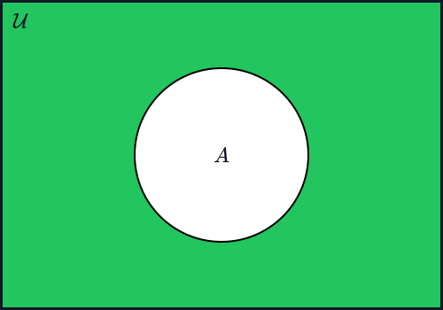
Since the complement of $A$ consists of everything in the universe that isn’t in $A$, the circle for $A$ itself is left unshaded, while everything else within the surrounding rectangle is shaded to represent $A^C$.
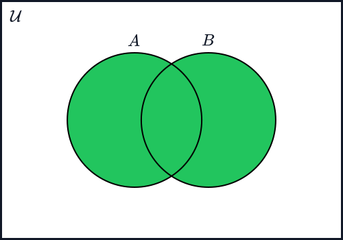
As long as an element is in $A$ or $B$, or even both, it’s included in the union — so both circles are shaded in their entirety, overlap included.
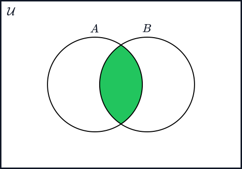
Here, only the sliver shared by both circles is shaded, since that’s the only region representing elements common to both $A$ and $B$.
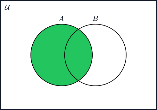
Only the part of $A$’s circle left over once the overlapping sliver shared with $B$ has been carved away is shaded.
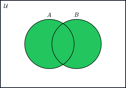
The symmetric difference shades everything covered by either circle except the overlapping sliver shared by both — everything a union would shade, minus whatever an intersection would shade.
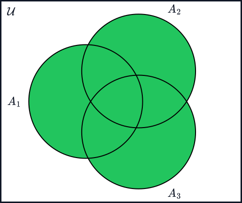
This same idea of shading extends naturally to more than two sets at once — every region covered by at least one of $A_1$, $A_2$, or $A_3$ is shaded to represent their multiple union.
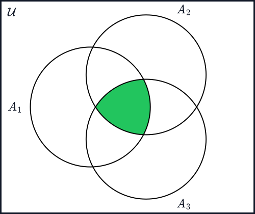
Here, only the single region shared by all three circles at once — where $A_1$, $A_2$, and $A_3$ all overlap — is shaded, representing their multiple intersection.
Understanding the laws of set theory is essential because they solve the problem of determining when two or more sets are equal, through fundamental equations including associativity, commutativity, and distribution. These laws provide a structured framework for defining and manipulating sets, ensuring consistency and precision in operations such as subset, difference, and symmetric difference.
In other words, by developing laws of set theory, we can essentially manipulate equations involving sets as if they were algebraic equations. In addition, the laws of set theory will allow us to convert complicated expressions involving sets into simpler ones, much like how we took complicated logical expressions and simplified them into smaller, logically equivalent expressions.
By studying these laws, one can formulate and prove mathematical concepts and theorems accurately. Furthermore, the foundations of many branches of mathematics are developed using the language of sets and set theory. In addition to the further development of mathematics, these laws also prove crucial to subjects like computer science and data science.
We’ve briefly described some aspects of set equality when we first introduced what sets were. We talked about how repetition and order are irrelevant with respect to what elements are contained within a set. As such, even if some elements are repeated in various descriptions, they still represent the same set.
However, as we’ve also seen, there are a wide variety of methods to describe a set and what elements are contained within it. Just because we come up with different descriptions, that doesn’t necessarily mean we’re describing different sets — sometimes we may be describing exactly the same set.
Consider the set
$$M = \{x \mid x \text{ is an even number between } -3 \text{ and } 10 \text{ inclusive}\}.$$We already know what elements are in $M$:
$$M = \{-2, 0, 2, 4, 6, 8, 10\}.$$Now consider the set
$$N = \{4x + 3 \mid x \in \{-1.25, -0.75, -0.25, 0.25, 0.75, 1.25, 1.75\}\}.$$The description of $N$ is a little more complicated, but we can still determine what elements are in $N$. The only tricky part is recognizing that the elements of $N$ are based off elements that are in the set $\{-1.25, -0.75, -0.25, 0.25, 0.75, 1.25, 1.75\}$, so we just have to iterate over those elements to figure out what’s in $N$. We’ll tabulate all values below:
\[ \begin{array}{l|l|l} x & 4x & 4x + 3 \\ \hline -1.25 & -5 & -2 \\ -0.75 & -3 & 0 \\ -0.25 & -1 & 2 \\ 0.25 & 1 & 4 \\ 0.75 & 3 & 6 \\ 1.25 & 5 & 8 \\ 1.75 & 7 & 10 \end{array} \]Since $N$ consists of the values $4x + 3$, we now know that
$$N = \{-2, 0, 2, 4, 6, 8, 10\}.$$Notice that $M$ and $N$ have the same number of elements ($7$), and all elements are exactly the same. Thus, since $M$ and $N$ represent the exact same set, we could write
$$M = N.$$It’s worth pointing out that since every element in $M$ is also in $N$, and every element in $N$ is also in $M$, we have that
\[ \begin{array}{rl} M &\subseteq N \\ N &\subseteq M \end{array} \]However, defining set equality by having the same elements isn’t exactly rigorous. Two sets can share some number of elements while also having different elements. As such, we don’t define set equality by simply having the same elements — instead, we look to the end of the previous example for inspiration.
Consider the two sets $A$ and $B$ taken from some universal set $\mathcal{U}$.
Sets $A$ and $B$ are called equal, and we write $A = B$, when
$$A \subseteq B$$and
$$B \subseteq A.$$This definition is precise because we can determine whether a set is a subset of another set under scrutiny. As such, because the definition of set equality requires we show two things to be true, proofs showing two sets to be equal are usually broken up into two parts.
It’s this definition of set equality that makes the next two theorems somewhat straightforward to prove.
For any $A, B \subseteq \mathcal{U}$, if $A \subseteq B$, then $A \cap B = A$.
Step 1: Show that $A \cap B \subseteq A$.
Let $x$ be an arbitrarily picked element within $A \cap B$ (meaning $x \in A \cap B$).
By definition, $x \in A$ and $x \in B$, and as such we know that $x \in A$.
Thus, we have shown that if $x \in A \cap B$, then $x \in A$. This means that $A \cap B \subseteq A$, completing Step 1.
Step 2: Show that $A \subseteq A \cap B$.
Let $x$ be an arbitrarily picked element of $A$. Because we have by premise that $A \subseteq B$, we also have that $x \in B$.
Thus, since $x \in A$ and $x \in B$, we have that $x \in A \cap B$ by definition.
We’ve just shown that when $x \in A$, we also have that $x \in A \cap B$. We then have by definition that $A \subseteq A \cap B$, completing Step 2.
Conclusion. Because we’ve shown that $A \subseteq A \cap B$ and that $A \cap B \subseteq A$, we have by definition that
$$A \cap B = A$$as desired.
Thus, by this theorem, whenever we know that $A \subseteq B$, we can replace $A \cap B$ with just $A$ anywhere we see $A \subseteq B$ in an equation. It’s worth stressing that we can only make such a replacement when we know $A \subseteq B$ — otherwise, doing so may not be correct.
There are a few more such equalities we can make use of, which we now show in the next theorem.
For any $A, B \subseteq \mathcal{U}$, we have that
$$(A \subseteq B) \Longleftrightarrow (A \cap B = A) \Longleftrightarrow (A \cup B = B) \Longleftrightarrow (B^C \subseteq A^C).$$We’ll break this proof up into four steps.
Step 1: $(A \subseteq B) \Longrightarrow (A \cap B = A)$.
This is simply the previous theorem.
Step 2: $(A \cap B = A) \Longrightarrow (A \cup B = B)$.
The premise of this logical implication is that $A \cap B = A$, so we can bring that fact in whenever needed.
First we show that $A \cup B \subseteq B$.
Let $x$ be an arbitrarily picked element in $A \cup B$. Thus, by definition, $x \in A$ or $x \in B$. If $x$ happens to be an element of $B$, then it’s tautologically true that $x \in B$.
If $x \in A$, then the premise tells us that $x \in A \cap B$, meaning $x \in B$ as well.
Either way, we have that whenever $x \in A \cup B$, we also have that $x \in B$, meaning $A \cup B \subseteq B$.
Second, we show that $B \subseteq A \cup B$.
Let $x$ be an arbitrarily picked element within $B$. Thus, because $x \in B$, we also have that $x \in A \cup B$.
We’ve just shown that whenever $x \in B$, we also have that $x \in A \cup B$. This means that $B \subseteq A \cup B$.
Finally, because we’ve shown that $A \cup B \subseteq B$ and $B \subseteq A \cup B$, we have that
$$A \cup B = B$$as desired.
Step 3: $(A \cup B = B) \Longrightarrow (B^C \subseteq A^C)$.
Remember that $A^C$ is the complement of $A$ within $\mathcal{U}$. Also remember that $A \cup B = B$ is a premise of this logical implication, so we can use that fact whenever we want (we can’t use $A \cap B = A$ as a premise here, since that isn’t included in the implication we’re considering).
We’re trying to show that $B^C \subseteq A^C$, so let $x$ be an arbitrarily picked element of $B^C$.
Because $x \in B^C$, we have by definition that $x \notin B$. Now, because $A \cup B = B$ and $x \notin B$, we also have that $x \notin A \cup B$.
Next, because $x \notin A \cup B$, we also know that $x \notin A$. Therefore, since $x \notin A$, we must have that $x \in A^C$.
We’ve just shown that whenever $x \in B^C$, we also have that $x \in A^C$ (assuming $A \cup B = B$ as a premise).
Thus by definition, whenever we know $A \cup B = B$, we have that $B^C \subseteq A^C$ as desired.
Step 4: $(B^C \subseteq A^C) \Longrightarrow (A \subseteq B)$.
We have $B^C \subseteq A^C$ as a premise, so we’ll invoke that fact when needed.
Let $x$ be an arbitrarily picked element of $A$. Since $x \in A$, we have by definition that $x \notin A^C$.
Now, because $B^C \subseteq A^C$ and $x \notin A^C$, we have (by Modus Tollens) that $x \notin B^C$.
Now, because $x \notin B^C$, we have by definition that $x \in B$.
Thus, we’ve shown that, assuming $B^C \subseteq A^C$ as a premise, whenever $x \in A$, we must also have that $x \in B$.
Therefore, assuming $B^C \subseteq A^C$ as a premise, we have that $A \subseteq B$ as desired.
Conclusion. Because we’ve shown that
\[ \begin{array}{l} (A \subseteq B) \Longrightarrow (A \cap B = A) \\[0.75em] (A \cap B = A) \Longrightarrow (A \cup B = B) \\[0.75em] (A \cup B = B) \Longrightarrow (B^C \subseteq A^C) \\[0.75em] (B^C \subseteq A^C) \Longrightarrow (A \subseteq B) \end{array} \]we have that they’re all logically equivalent, meaning we have that
$$(A \subseteq B) \Longleftrightarrow (A \cap B = A) \Longleftrightarrow (A \cup B = B) \Longleftrightarrow (B^C \subseteq A^C)$$as desired.
Because of this theorem, whenever we know one of
$$A \subseteq B \qquad A \cap B = A \qquad A \cup B = B \qquad B^C \subseteq A^C$$is true, we automatically know that the other three are true as well.
The total opposite of two sets $A$ and $B$ being equal is when $A$ and $B$ have absolutely no elements in common. Of course, if two sets share no element in common, then their intersection is a set with no elements in it — the empty set.
Consider the two sets $A$ and $B$ taken from some universal set $\mathcal{U}$.
$A$ and $B$ are called disjoint whenever
$$A \cap B = \emptyset.$$Many of the concepts discussed so far may seem disparate. However, they’re more connected than may initially appear.
Let $A, B \subseteq \mathcal{U}$.
$$(A \cap B = \emptyset) \Longleftrightarrow (A \cup B = A \triangle B)$$Because we have a logical biconditional, we break this proof into two steps. First, we assume $A \cap B = \emptyset$ as a premise and show that $A \cup B = A \triangle B$. Next, we assume $A \cup B = A \triangle B$ as a premise and show that $A \cap B = \emptyset$.
Step 1: $(A \cap B = \emptyset) \Longrightarrow (A \cup B = A \triangle B)$.
First, we try to show that $A \cup B \subseteq A \triangle B$.
Let $x$ be an arbitrarily picked element within $A \cup B$. Thus, we have by definition that $x \in A$ or $x \in B$, but because $A \cap B = \emptyset$, $x$ can’t be in both $A$ and $B$.
Thus we either have that $x \in A$ and $x \notin B$, meaning $x \in A \triangle B$, or we have that $x \notin A$ and $x \in B$, meaning we still have that $x \in A \triangle B$.
Either way, we have that $x \in A \triangle B$. Hence, we’ve just shown that (assuming $A \cap B = \emptyset$) whenever $x \in A \cup B$, we also have that $x \in A \triangle B$ as well, and so we have that
$$A \cup B \subseteq A \triangle B.$$Second, we try to show that $A \triangle B \subseteq A \cup B$.
Now, let $x$ be an arbitrarily picked element in $A \triangle B$. Thus, by definition, either $x \in A$ and $x \notin B$, meaning $x \in A \cup B$, or $x \notin A$ and $x \in B$, meaning $x \in A \cup B$.
Either way, we know that whenever $x \in A \triangle B$, we also know that $x \in A \cup B$ as well.
Thus, by definition we have that
$$A \triangle B \subseteq A \cup B.$$Finally, because we know that $A \cup B \subseteq A \triangle B$ and $A \triangle B \subseteq A \cup B$, we have by definition that
$$A \cup B = A \triangle B.$$This shows that $(A \cap B = \emptyset) \Longrightarrow (A \cup B = A \triangle B)$, completing Step 1.
Step 2: $(A \cap B = \emptyset) \Longleftarrow (A \cup B = A \triangle B)$.
Here, we’re assuming $A \cup B = A \triangle B$ as a premise, and are trying to show that $A \cap B = \emptyset$.
Because we know that $A \cup B = A \triangle B$, we have by the definition of set equality that $A \cup B \subseteq A \triangle B$ and $A \triangle B \subseteq A \cup B$.
Thus, for any element $x \in A \cup B$, we also know that $x \in A \triangle B$. However, since $x \in A \triangle B$, we know that either
$$x \in A \text{ and } x \notin B \qquad \text{or} \qquad x \notin A \text{ and } x \in B.$$Either way, no element $x \in A \cup B$ can be in both $A$ and $B$.
Thus, because no element $x$ exists such that $x \in A \cap B$, we must have that $A \cap B$ is empty, meaning $A \cap B = \emptyset$.
This shows that $(A \cup B = A \triangle B) \Longrightarrow (A \cap B = \emptyset)$, completing Step 2.
Conclusion. Because we’ve shown that $(A \cap B = \emptyset) \Longrightarrow (A \cup B = A \triangle B)$ and $(A \cup B = A \triangle B) \Longrightarrow (A \cap B = \emptyset)$, we must have that
$$(A \cap B = \emptyset) \Longleftrightarrow (A \cup B = A \triangle B)$$as desired.
This theorem connects the concepts of equal sets, disjoint sets, unions, and symmetric differences.
Remember that $x \in A$ is a statement about $x$ being a member of set $A$. Because it’s a statement, it has a truth value of either $0$ or $1$.
One powerful tool we had at our disposal for analyzing logical expressions was a truth table. We can adapt truth tables to analyze set relationships as well. In this case, membership tables offer a tabular way of representing element arguments.
\[ \begin{array}{l|l|l|l} x \in A & x \in B & x \in A \cup B & x \in A \cap B \\ \hline 0 & 0 & 0 & 0 \\ 0 & 1 & 1 & 0 \\ 1 & 0 & 1 & 0 \\ 1 & 1 & 1 & 1 \end{array} \]Instead of using some generic symbol for a generic object whose membership in some set we want to analyze, we could simply list whatever sets we’re analyzing. As such, we could rewrite the above table like so:
\[ \begin{array}{l|l|l|l} A & B & A \cup B & A \cap B \\ \hline 0 & 0 & 0 & 0 \\ 0 & 1 & 1 & 0 \\ 1 & 0 & 1 & 0 \\ 1 & 1 & 1 & 1 \end{array} \]All of the set operations have their corresponding tables, which we can include inside one large table:
\[ \begin{array}{l|l|l|l|l|l|l} A & B & A^C & A \cup B & A \cap B & A - B & A \triangle B \\ \hline 0 & 0 & 1 & 0 & 0 & 0 & 0 \\ 0 & 1 & 1 & 1 & 0 & 0 & 1 \\ 1 & 0 & 0 & 1 & 0 & 1 & 1 \\ 1 & 1 & 0 & 1 & 1 & 0 & 0 \end{array} \]Based on the values above, we see that there are obvious analogues with logical operators:
\[ \begin{array}{rl} A^C &\text{ pairs with } \neg a \\ A \cup B &\text{ pairs with } a \lor b \\ A \cap B &\text{ pairs with } a \land b \\ A - B &\text{ pairs with } \neg(a \to b) \\ A \triangle B &\text{ pairs with } a \veebar b \end{array} \]Notice that the set difference resembles the logical complement of an implication.
In addition to the set operations, we can determine subset relationships. Let’s take a look at one more table to see an example:
\[ \begin{array}{l|l|l|l|l|l} x \in A & x \in B & x \in A \cup B & x \in A \cap B & (x \in A \cap B) \to (x \in A) & (x \in A) \to (x \in A \cup B) \\ \hline 0 & 0 & 0 & 0 & 1 & 1 \\ 0 & 1 & 1 & 0 & 1 & 1 \\ 1 & 0 & 1 & 0 & 1 & 1 \\ 1 & 1 & 1 & 1 & 1 & 1 \end{array} \]Notice that the columns $(x \in A \cap B) \to (x \in A)$ and $(x \in A) \to (x \in A \cup B)$ have all $1$s. As such, we can write
$$(x \in A \cap B) \Longrightarrow (x \in A) \qquad \text{and} \qquad (x \in A) \Longrightarrow (x \in A \cup B)$$which is exactly the definition of subset. As such, we can determine that a set $A$ is a subset of some other set $B$ by comparing their respective columns. If $A$ has $1$s in every row where $B$ also has a $1$, then we know that $A \subseteq B$.
Let’s prove a simple observation we may have had in our study of set relationships and operations.
Let $A, B \subseteq \mathcal{U}$.
$$(A \cap B) \subseteq A \subseteq (A \cup B)$$Let’s examine a membership table:
\[ \begin{array}{l|l|l|l} A & B & A \cup B & A \cap B \\ \hline 0 & 0 & 0 & 0 \\ 0 & 1 & 1 & 0 \\ 1 & 0 & 1 & 0 \\ 1 & 1 & 1 & 1 \end{array} \]Now, we can compare specific columns we want, but we’ll do so in two separate membership tables:
\[ \begin{array}{l|l} A \cap B & A \\ \hline 0 & 0 \\ 0 & 0 \\ 0 & 1 \\ 1 & 1 \end{array} \qquad \begin{array}{l|l} A & A \cup B \\ \hline 0 & 0 \\ 0 & 1 \\ 1 & 1 \\ 1 & 1 \end{array} \]In the table on the left, every row of $A \cap B$ that has a $1$ also has a $1$ in the $A$ column. As such, we know that $(A \cap B) \subseteq A$.
Additionally, from the table on the right, every row in the $A$ column that has a $1$ also has a $1$ in the $A \cup B$ column. As such, we know that $A \subseteq (A \cup B)$.
Because we know that $(A \cap B) \subseteq A$ and $A \subseteq (A \cup B)$, we can combine them into the single expression
$$(A \cap B) \subseteq A \subseteq (A \cup B)$$as desired.
Membership tables can be a convenient way to represent an element argument in tabular form. However, membership tables won’t totally replace element arguments, as sometimes the element argument is simpler to make for more esoteric situations where tables can be cumbersome to use.
We’ve already examined a number of simple laws (referred to as theorems) above, and have demonstrated their truth by way of element arguments and membership tables. What’s demonstrated above only scratches the surface of the multitude of equal-set relationships we can exploit. Below, we present a large table offering even more such laws.
As you look over this table, it would be wise to compare it with the table presented in Chapter 1, Section 5. You should see many analogues.
For any sets $A$, $B$, and $C$ taken from some universal set $\mathcal{U}$, we have the following equivalencies:
| Law of Double Complement | $(A^C)^C = A$ |
| DeMorgan’s Laws | $\begin{array}{c} (A \cup B)^C = A^C \cap B^C \\ (A \cap B)^C = A^C \cup B^C \end{array}$ |
| Commutative Laws | $\begin{array}{c} A \cup B = B \cup A \\ A \cap B = B \cap A \end{array}$ |
| Associative Laws | $\begin{array}{c} A \cup (B \cup C) = (A \cup B) \cup C \\ A \cap (B \cap C) = (A \cap B) \cap C \end{array}$ |
| Distributive Laws | $\begin{array}{c} A \cup (B \cap C) = (A \cup B) \cap (A \cup C) \\ A \cap (B \cup C) = (A \cap B) \cup (A \cap C) \end{array}$ |
| Idempotent Laws | $\begin{array}{c} A \cup A = A \\ A \cap A = A \end{array}$ |
| Identity Laws | $\begin{array}{c} A \cup \emptyset = A \\ A \cap \mathcal{U} = A \end{array}$ |
| Inverse Laws | $\begin{array}{c} A \cup A^C = \mathcal{U} \\ A \cap A^C = \emptyset \end{array}$ |
| Domination Laws | $\begin{array}{c} A \cup \mathcal{U} = \mathcal{U} \\ A \cap \emptyset = \emptyset \end{array}$ |
| Absorption Laws | $\begin{array}{c} A \cup (A \cap B) = A \\ A \cap (A \cup B) = A \end{array}$ |
Certainly, many more such laws and equivalencies exist, but the table above represents some of the more ubiquitous laws that are often used.
These laws present us an opportunity to directly compare three different proof techniques. First, we use a membership table.
For any $A \subseteq \mathcal{U}$,
$$(A^C)^C = A$$General Strategy: We’ll use a membership table to compare the columns for $A$ and $(A^C)^C$.
\[ \begin{array}{l|l|l} A & A^C & (A^C)^C \\ \hline 0 & 1 & 0 \\ 1 & 0 & 1 \end{array} \]Since the columns for $A$ and $(A^C)^C$ are exactly the same, they’re equal, and so we have
$$A = (A^C)^C$$as desired.
Now, compare such a simple strategy with a standard element argument used in the next proof.
For any $A, B \subseteq \mathcal{U}$,
\[ \begin{array}{rl} (A \cup B)^C &= A^C \cap B^C \\ (A \cap B)^C &= A^C \cup B^C \end{array} \]General Strategy: We’ll split this proof up into two steps, where each step is dedicated to a different part of DeMorgan’s Laws. Both steps will make use of standard element arguments, as well as the definition of set equality.
Step 1: $(A \cup B)^C = A^C \cap B^C$.
First, we show that $(A \cup B)^C \subseteq A^C \cap B^C$.
Suppose that element $x \in \mathcal{U}$ was also in $(A \cup B)^C$, meaning $x \in (A \cup B)^C$.
Since $x \in (A \cup B)^C$, we know that $x \notin ((A \cup B)^C)^C$, and by the Law of Double Complement, we also know that $x \notin A \cup B$.
Now we simultaneously know that $x \notin A$ (otherwise $x$ would be in $A \cup B$, which we just established isn’t the case) and $x \notin B$ (again, because then $x$ would be in $A \cup B$).
Thus, since $x \notin A$ and $x \notin B$, we know that $x \in A^C$ and $x \in B^C$, meaning $x \in A^C \cap B^C$, which is what we’re trying to show.
Thus, whenever we have that $x \in (A \cup B)^C$, we know that $x \in A^C \cap B^C$, meaning
$$(A \cup B)^C \subseteq A^C \cap B^C.$$Second, we show that $A^C \cap B^C \subseteq (A \cup B)^C$.
Now, suppose we knew that $x \in A^C \cap B^C$. Thus we simultaneously know that $x \in A^C$ and $x \in B^C$.
This means we have that $x \notin A$ and $x \notin B$. Thus, since $x$ is in neither $A$ nor $B$, $x$ can’t possibly be in $A \cup B$, meaning $x \notin A \cup B$. This means that $x \in (A \cup B)^C$.
Thus, whenever we know that $x \in A^C \cap B^C$, we also know that $x \in (A \cup B)^C$, which means we have that
$$A^C \cap B^C \subseteq (A \cup B)^C.$$Finally, because we’ve shown that $(A \cup B)^C \subseteq A^C \cap B^C$ and $A^C \cap B^C \subseteq (A \cup B)^C$, we have by definition that
$$(A \cup B)^C = A^C \cap B^C$$as desired.
Step 2: $(A \cap B)^C = A^C \cup B^C$.
Using nearly the exact same process as was used in Step 1, we come to the conclusion that
$$(A \cap B)^C = A^C \cup B^C.$$Conclusion. By now, we’ve shown that both $(A \cup B)^C = A^C \cap B^C$ and $(A \cap B)^C = A^C \cup B^C$, and as such have completely established DeMorgan’s Laws.
The last of these laws we’ll prove in this section will be the Distributive Laws. Instead of making two separate element arguments to establish that $A \cup (B \cap C) \subseteq (A \cup B) \cap (A \cup C)$ and $(A \cup B) \cap (A \cup C) \subseteq A \cup (B \cap C)$, we’ll use logical equivalencies to show that $A \cup (B \cap C)$ and $(A \cup B) \cap (A \cup C)$ are subsets of each other simultaneously.
For any $A, B, C \subseteq \mathcal{U}$,
\[ \begin{array}{rl} A \cup (B \cap C) &= (A \cup B) \cap (A \cup C) \\ A \cap (B \cup C) &= (A \cap B) \cup (A \cap C) \end{array} \]General Strategy: We’ll use logical equivalencies to show that any element of $A \cup (B \cap C)$ is also an element of $(A \cup B) \cap (A \cup C)$. Since we use logical equivalencies, this also applies the other way simultaneously.
\[ \begin{array}{lll} & \boldsymbol{x \in A \cup (B \cap C)} & \textbf{Reason} \\ \Longleftrightarrow & (x \in A) \lor (x \in B \cap C) & \text{Definition of Set Union} \\ \Longleftrightarrow & (x \in A) \lor [(x \in B) \land (x \in C)] & \text{Definition of Set Intersection} \\ \Longleftrightarrow & [(x \in A) \lor (x \in B)] \land [(x \in A) \lor (x \in C)] & \text{Distribution of } \lor \text{ over } \land \\ \Longleftrightarrow & (x \in A \cup B) \land (x \in A \cup C) & \text{Definition of Set Union} \\ \Longleftrightarrow & x \in (A \cup B) \cap (A \cup C) & \text{Definition of Set Intersection} \end{array} \]We’ve just established that
$$(x \in A \cup (B \cap C)) \Longleftrightarrow (x \in (A \cup B) \cap (A \cup C)).$$Thus, whenever $x \in A \cup (B \cap C)$, we also simultaneously know that $x \in (A \cup B) \cap (A \cup C)$. As such, we know that
$$A \cup (B \cap C) \subseteq (A \cup B) \cap (A \cup C) \qquad \text{and} \qquad (A \cup B) \cap (A \cup C) \subseteq A \cup (B \cap C)$$are simultaneously true, and so we have that
$$A \cup (B \cap C) = (A \cup B) \cap (A \cup C)$$as desired. The same logic also shows that $A \cap (B \cup C) = (A \cap B) \cup (A \cap C)$ as well.
Of course, the rest of the Laws of Set Theory can be proven in many different ways. Because it’s a good exercise to provide a proof for all the above laws, proofs for the remaining laws are asked for in this chapter’s practice questions.
Just as we can use the Laws of Logic to simplify complicated logical expressions, we can also use the Laws of Set Theory to simplify complicated expressions involving sets.
Suppose we were dealing with the expression
$$X \cap (Y - X)$$where $X, Y \subseteq \mathcal{U}$.
We can simplify the above expression in the following way:
\[ \begin{array}{lll} & \boldsymbol{X \cap (Y - X)} & \textbf{Reason} \\ = & X \cap (Y \cap X^C) & \text{Definition of Set Difference} \\ = & X \cap (X^C \cap Y) & \text{Commutative Law} \\ = & (X \cap X^C) \cap Y & \text{Associative Law} \\ = & \emptyset \cap Y & \text{Inverse Law} \\ = & \emptyset & \text{Domination Law} \end{array} \]Thus, we’ve just established that for any $X, Y \subseteq \mathcal{U}$,
$$X \cap (Y - X) = \emptyset.$$We made use of an additional law of Set Theory above, where we can express the set difference operation using only intersection and complement:
$$Y - X = Y \cap X^C.$$We’ll now justify that equality:
\[ \begin{array}{lll} & \boldsymbol{Y - X} & \textbf{Reason} \\ = & \{p \mid (p \in Y) \land (p \notin X)\} & \text{Definition of Set Difference} \\ = & \{p \mid (p \in Y) \land (p \in X^C)\} & \text{Definition of Set Complement} \\ = & Y \cap X^C & \text{Definition of Set Intersection} \end{array} \]For any two sets $A$ and $B$ taken from some universal set $\mathcal{U}$, we have that
$$A - B = A \cap B^C.$$As a matter of fact, we can also express the symmetric difference operation using only union, intersection, and complement, which we justify below:
\[ \begin{array}{lll} & \boldsymbol{Y \triangle X} & \textbf{Reason} \\ = & \{p \mid (p \in Y) \veebar (p \in X)\} & \text{Definition of Symmetric Difference} \\ = & \{p \mid ((p \in Y) \land (p \notin X)) \lor ((p \notin Y) \land (p \in X))\} & \text{Definition of Logical Exclusive-or} \\ = & \{p \mid ((p \in Y) \land (p \in X^C)) \lor ((p \in Y^C) \land (p \in X))\} & \text{Definition of Set Complement} \\ = & \{p \mid (p \in Y \cap X^C) \lor (p \in Y^C \cap X)\} & \text{Definition of Set Intersection} \\ = & (Y \cap X^C) \cup (Y^C \cap X) & \text{Definition of Set Union} \end{array} \]For any two sets $A$ and $B$ taken from some universal set $\mathcal{U}$, we have that
$$A \triangle B = (A \cap B^C) \cup (B^C \cap A).$$This just goes to show how important the union, intersection, and complement operations are when it comes to sets, because no matter how we want to combine any combination of sets, we can always do so using just those three operations.
Can we rewrite the expression
$$(X - Y)^C$$using only union, intersection, and complement? Let’s try and see.
\[ \begin{array}{lll} & \boldsymbol{(X - Y)^C} & \textbf{Reason} \\ = & (X \cap Y^C)^C & \text{Definition of Set Difference} \\ = & X^C \cup (Y^C)^C & \text{DeMorgan's Law} \\ = & X^C \cup Y & \text{Law of Double Complement} \end{array} \]So $(X - Y)^C$ is equivalent to $X^C \cup Y$.
We can simplify the expression
$$(((X \cup Y) \cap Z)^C \cup Y)^C$$using the following steps:
\[ \begin{array}{lll} & \boldsymbol{(((X \cup Y) \cap Z)^C \cup Y)^C} & \textbf{Reason} \\ = & (((X \cup Y) \cap Z)^C)^C \cap (Y^C)^C & \text{DeMorgan's Law} \\ = & ((X \cup Y) \cap Z) \cap Y & \text{Law of Double Complement} \\ = & (Z \cap (X \cup Y)) \cap Y & \text{Commutative Law} \\ = & Z \cap ((X \cup Y) \cap Y) & \text{Associative Law} \\ = & Z \cap ((X \cap Y) \cup (Y \cap Y)) & \text{Distributive Law} \\ = & Z \cap ((X \cap Y) \cup Y) & \text{Idempotent Law} \\ = & Z \cap (Y \cup (X \cap Y)) & \text{Commutative Law} \\ = & Z \cap Y & \text{Absorption Law} \end{array} \]We’ve seen DeMorgan’s Laws applied to two sets at a time. Let’s see what happens when we have three sets at a time:
\[ \begin{array}{lll} & \boldsymbol{(A \cup B \cup C)^C} & \textbf{Reason} \\ = & ((A \cup B) \cup C)^C & \text{Associative Law} \\ = & (A \cup B)^C \cap C^C & \text{DeMorgan's Laws} \\ = & A^C \cap B^C \cap C^C & \text{DeMorgan's Laws} \end{array} \]It stands to reason that repeated applications of DeMorgan’s Laws would work for intersection as well.
Furthermore, no matter how many sets we have, it seems as if we can just repeatedly apply DeMorgan’s Laws and the Associative Law. Based on this observation, we make the following observations, where $I$ is an index set over which the multiple union or intersection is taken:
\[ \begin{array}{rl} \left(\bigcup_{i \in I} A_i\right)^C &= \bigcap_{i \in I} A_i^C \\[0.75em] \left(\bigcap_{i \in I} A_i\right)^C &= \bigcup_{i \in I} A_i^C \end{array} \]Of course, mere intuition doesn’t prove anything to be true. Instead, we must rely on rigorous tools, such as element arguments and logical equivalencies, to establish truth without any doubt.
For a universal set $\mathcal{U}$ and index set $I$, the following equalities hold:
\[ \begin{array}{rl} \left(\bigcup_{i \in I} A_i\right)^C &= \bigcap_{i \in I} A_i^C \\[0.75em] \left(\bigcap_{i \in I} A_i\right)^C &= \bigcup_{i \in I} A_i^C \end{array} \]General Strategy: We’ll make use of various definitions of Set Theory, including Complement. We also make use of the logical rules that apply when negating quantified statements, as discussed in Chapter 1, Section 10.
\[ \begin{array}{lll} & \boldsymbol{x \in \left(\bigcup_{i \in I} A_i\right)^C} & \textbf{Reason} \\ \Longleftrightarrow & x \notin \bigcup_{i \in I} A_i & \text{Definition of Set Complement} \\ \Longleftrightarrow & \neg \exists i \in I\ [x \in A_i] & \text{Definition of Multiple Union} \\ \Longleftrightarrow & \forall i \in I\ [x \notin A_i] & \text{Negating a Quantified Statement} \\ \Longleftrightarrow & \forall i \in I\ [x \in A_i^C] & \text{Definition of Set Complement} \\ \Longleftrightarrow & x \in \bigcap_{i \in I} A_i^C & \text{Definition of Multiple Intersection} \end{array} \]We’ve just shown why the first equivalence is true. By similar logic, the second is also shown to be true. This establishes both equivalencies as desired.
The generalized versions of DeMorgan’s Laws will prove extremely useful in our further study of math.
All of the proof techniques discussed thus far work on sets that have infinitely many elements. For example, we’ve talked about theorems that apply to all even numbers, not merely some of them. For example, for all even numbers, adding one yields an odd number. As another example, no matter which two even numbers are added together, the sum is always another even number.
We’ve even talked about theorems that apply to all sets in general, not merely some of them. These include the set operations and the set equalities.
It’s not hard to see why methods that apply to sets of infinitely many objects are powerful. On the other hand, there may be times when there are only a finite number of objects we’re interested in examining. Here, we discuss a method for proving theorems dealing with only a finite number of elements.
Admittedly, dealing with only a finite number of elements seems hardly useful, as we mostly want results that apply generally, and not specifically. Here, we provide a contrived example simply to demonstrate the technique.
Suppose we wanted to prove that the integers in the set
$$E = \{2, 4, 6, 8, 10, 12, 14, 16, 18, 20\}$$could all be expressed as a sum of no more than three perfect squares. We could do this by simply tabulating the results.
\[ \begin{array}{l|l} n & \text{Sum of squares} \\ \hline 2 & 1^2 + 1^2 \\ 4 & 2^2 \\ 6 & 1^2 + 1^2 + 2^2 \\ 8 & 2^2 + 2^2 \\ 10 & 1^2 + 3^2 \\ 12 & 2^2 + 2^2 + 2^2 \\ 14 & 1^2 + 2^2 + 3^2 \\ 16 & 4^2 \\ 18 & 3^2 + 3^2 \\ 20 & 2^2 + 4^2 \end{array} \]As such, we’ve “proved” the desired fact.
Notice that we didn’t say the numbers in $E$ could be written as a unique sum. There may be more than one way to write some of the numbers as a sum of perfect squares, like in the following example:
$$18 = 1^2 + 1^2 + 4^2.$$We could perhaps call the result derived in the previous example a theorem, since we did provide a proof for the fact, but we prefer to reserve the term theorem for “major” results. That result was merely an exercise.
Based on the previous example, we can see why the method presented in this section is called the Method of Exhaustion: it’s because we exhaustively check every single element in the desired set for a desired property. Note that while the term exhaustion is used to describe the thoroughness of checking every element, it doesn’t necessarily refer to the feeling one may get whilst performing the checking — though it should be said that for rather large sets, this method can be tiresome.
Let’s lay out the argument in logical fashion, same as we’ve done before. The reason this method works is because we verify that every element in the desired set has some desired property.
Suppose set $A$ is a finite subset consisting of the $n$ elements
$$A = \{a_1, a_2, a_3, \dots, a_n\}$$taken from some universal set $\mathcal{U}$. Furthermore, suppose $p$ is an open statement defined on $\mathcal{U}$. The Method of Exhaustion is simply an argument of the form
\[ \begin{array}{l} p(a_1) \\ p(a_2) \\ p(a_3) \\ \vdots \\ p(a_n) \\ \hline \therefore \forall x \in A\ [p(x)] \end{array} \]That’s all there really is to it.
Just because a set is finite doesn’t mean it’s feasible to hand-check every single element within it. Sometimes tasks can be automated by writing computer programs to check thousands or even millions of elements in a timely fashion.
While the example presented above was rather contrived, one major result proved using the Method of Exhaustion was the Four Color Theorem. This theorem states that any planar (basically meaning flat) map only needs at most four different colors so that no adjacent regions on the map share the same color. For centuries, cartographers have been making maps of various places around the world, and one way to draw maps is to color regions so they’re easily distinguishable. It’s typically expected that adjacent regions on a map are colored differently, helping them stand out visually.
It was shown at some point in the late 1800s that no more than five colors were needed for any map so that no adjacent regions shared a color, but it was suspected that no more than four colors were needed as well. Though many mathematicians attempted to prove that no more than four colors were needed, many efforts proved fruitless.
Progress marched forward in the 1960s with the advent of computing technology. Two mathematicians, Kenneth Appel and Wolfgang Haken, further developed results derived from Heinrich Heesch to complete a proof. Essentially, one major step in the proof was showing that all maps could be “reduced” to a small number of essential configurations (basically, all maps are distortions of some simpler underlying map that represent the same types of regions). Appel and Haken found that there were only $1834$ such configurations.
Once Appel and Haken found these configurations, it was simply a matter of checking each and every one of them — using the Method of Exhaustion.
This proof was the first major proof to be verified by computer. As such, it was a controversial result: not all mathematicians readily accepted the proof, because it was hard and time-consuming for a human to check.
Nevertheless, the proof has mostly withstood scrutiny, with a minor error being corrected by Appel and Haken sometime in the late 1980s.
The point is that while the Method of Exhaustion may seem overly simple and contrived, being restricted to only finite sets instead of infinite sets, it’s still a valid proof technique that can come in handy.
When working with a set of related objects, we may want to split that set up into smaller, more manageable sets.
For example, we may want to split up the integers based on parity: even integers, and odd integers. When dealing with the real numbers, we may want to split them up into three separate sets: the positive real numbers, the negative real numbers, and the number $0$. One more example may be the positive rational numbers, where we split them up based on how big they are — we may have all of the positive rational numbers less than $1$ in one set, and all of the positive rational numbers greater than or equal to $1$ in the other set.
No matter how we split up a set, we’ll want to make sure that all elements of the original set are accounted for in one of the smaller subsets we form.
In the introduction to this section, we mentioned three examples of how we may split a large set into smaller subsets, making sure every element within the original set is in one of the subsets. A partition of a set creates these subsets while making sure that every element is accounted for; however, the word partition also invokes the idea of separation — no two subsets should share any elements. The following definition of partition offers something more precise.
Consider some set $A \subseteq \mathcal{U}$ along with some index set $I$.
For each $i \in I$, let $A_i \subseteq A$ such that $A_i \neq \emptyset$. Then the set
$$\{A_i \mid i \in I\}$$is called a partition of $A$ if (and only if) the following two conditions are satisfied:
\[ \begin{array}{rl} \text{(1)} &\bigcup_{i \in I} A_i = A \\[0.75em] \text{(2)} &\forall i, j \in I\ [(i \neq j) \to (A_i \cap A_j = \emptyset)] \end{array} \]Note that none of the sets in the partition can be empty. The whole point of forming a partition is to take elements from the original set and put them into a subset.
Consider the following set of numbers:
$$A = \{0, 1, -1, 2, -2, 3, -3, 4, -4\}.$$If we want to partition this set, we need to form non-empty subsets that are all disjoint, and such that all elements in $A$ are in one of the subsets.
Here’s one way to partition $A$:
\[ \begin{array}{rl} A_1 &= \{0, 1\} \\ A_2 &= \{-1, 2, -2\} \\ A_3 &= \{3, -3, 4, -4\} \end{array} \]Notice that we didn’t start with the index set $I = \{1, 2, 3\}$. Instead, we formed the subsets first, and then indexed them. Of course, we should check to see if the conditions specified in the definition are met:
\[ \begin{array}{lll} \boldsymbol{A_1 \cup A_2 \cup A_3} & = & \{0, 1\} \cup \{-1, 2, -2\} \cup \{3, -3, 4, -4\} \\ = & A & \end{array} \]This means that every element from $A$ was accounted for. Now we check to see if all the subsets are disjoint:
\[ \begin{array}{rl} A_1 \cap A_2 &= \{0, 1\} \cap \{-1, 2, -2\} = \emptyset \\ A_1 \cap A_3 &= \{0, 1\} \cap \{3, -3, 4, -4\} = \emptyset \\ A_2 \cap A_3 &= \{-1, 2, -2\} \cap \{3, -3, 4, -4\} = \emptyset \end{array} \]Both conditions have been met, so this is a legitimate partition of $A$.
There are other ways to partition the set
$$A = \{0, 1, -1, 2, -2, 3, -3, 4, -4\}.$$One such way to partition the set is with the following:
\[ \begin{array}{rl} X_1 &= \{0, 4\} \\ X_2 &= \{-1\} \\ X_3 &= \{1, 2\} \\ X_4 &= \{-2, -3, -4\} \\ X_5 &= \{3\} \end{array} \]Notice that we didn’t use the letter $A$ for the names of these subsets. The important thing is the content of the subsets themselves, not the name given to them. As long as the two conditions are met, the collection of sets forms a partition. We could also put every element of $A$ into its own subset, like so:
\[ \begin{array}{rl} Y_1 &= \{0\} \\ Y_2 &= \{1\} \\ Y_3 &= \{-1\} \\ Y_4 &= \{2\} \\ Y_5 &= \{-2\} \\ Y_6 &= \{3\} \\ Y_7 &= \{-3\} \\ Y_8 &= \{4\} \\ Y_9 &= \{-4\} \end{array} \]Yet another partition we could form is just by taking the entire set itself:
$$Z = \{0, 1, -1, 2, -2, 3, -3, 4, -4\}.$$Since there are no other sets in this partition, it’s trivially true that the union of all the sets forms $A$. Furthermore, since there are no other sets in the partition, it’s trivially true that all sets in the partition are disjoint.
As mentioned in the introduction, one thing we can do is split up the integers into two subsets: one containing the even integers, and a second subset containing the odd integers.
\[ \begin{array}{rl} A &= \{0, 2, -2, 4, -4, 6, -6, \dots\} \\ B &= \{1, -1, 3, -3, 5, -5, 7, -7, \dots\} \end{array} \]Here, we didn’t use the same letter for the subset names, nor did we use indices. Again, the names of the subsets aren’t important. What’s important is knowing that all subsets are mutually disjoint, and that all elements from the original set are accounted for.
One way to partition the real numbers $\mathbb{R}$ is into three subsets: the subset of all positive real numbers greater than $0$, the subset of all negative real numbers less than $0$, and finally the subset containing just the number $0$.
\[ \begin{array}{rl} X &= \{x \in \mathbb{R} \mid x < 0\} \\ Y &= \{0\} \\ Z &= \{x \in \mathbb{R} \mid x > 0\} \end{array} \]Some numbers that are in $X$ include $-\pi$, $-12.3372$, and $-\sqrt{2}$.
Some numbers in $Z$ include $1.2345$, $12$, and $\pi \cdot \pi$.
As one more example, we could partition the positive rational numbers into two separate subsets.
\[ \begin{array}{rl} A &= \left\{\frac{a}{b} \ \middle|\ (a \in \{0, 1, 2, 3, \dots\}) \land (b \in \{1, 2, 3, \dots\}) \land \left(\frac{a}{b} < 1\right)\right\} \\ B &= \left\{\frac{a}{b} \ \middle|\ (a \in \{0, 1, 2, 3, \dots\}) \land (b \in \{1, 2, 3, \dots\}) \land \left(\frac{a}{b} \geq 1\right)\right\} \end{array} \]Previously, we talked about a proof technique where we examine every single element of a finite set. In a sense, we examined multiple cases, and verified some result for each of those cases. An exhaustive proof is a special kind of proof by casework.
Sometimes, we may have trouble demonstrating that some result holds for a set of elements. However, if we partition the set into groups that have their own special traits, and those traits make it easy to show the desired result holds, a proof by casework can be used to establish the desired result for the entire set.
Suppose we were trying to prove a statement of the form
$$p \to c.$$Suppose that we somehow knew that
$$p = p_1 \lor p_2 \lor p_3 \lor \dots \lor p_n.$$If we knew how to show that
\[ \begin{array}{l} p_1 \to c \\ p_2 \to c \\ p_3 \to c \\ \vdots \\ p_n \to c \end{array} \]we would then have that
$$(p_1 \lor p_2 \lor p_3 \lor \dots \lor p_n) \to c.$$Thus, because $p = p_1 \lor p_2 \lor p_3 \lor \dots \lor p_n$, we would also have that $p \to c$ by extension.
This proof technique is simply an extension of the Rule of Proof by Cases:
\[ \begin{array}{l} p \to r \\ q \to r \\ \hline \therefore (p \lor q) \to r \end{array} \]as presented in Chapter 2, Section 6. Even though we could have discussed this proof technique in Chapter 2, we decided to hold off until partitions were discussed, because a lot of casework is done by considering elements from disjoint sets. However, when doing casework, it’s not important that elements from the universe of discourse are in only one subset of a partition.
Whether we form a partition of the universe, or we split the universe up into overlapping subsets, isn’t important. What’s important is that, once we have our desired subsets, every element is represented by at least one of those subsets.
When we partition a set, we split it into disjoint subsets where every element is accounted for in one of the subsets. We don’t have to form these subsets arbitrarily. Instead, we could take all elements from the original set that have some common property, and stick those elements into a subset. We can repeat this process until all elements are accounted for.
Then, from each of these subsets, we choose an arbitrary element. Then, whatever is true of that element will be true for all elements within that subset. In essence, we’re using the principles of Universal Specification and Universal Generalization, along with a partition, to prove a theorem.
Our first theorem will be a result about absolute values of real numbers. As a reminder, here’s the definition of absolute value of a real number.
For any real number $x$, the absolute value of $x$, commonly denoted $|x|$, is the non-negative real number given by the following:
\[ \begin{array}{rl} |x| = x & \text{when } x \geq 0 \\ |x| = -x & \text{when } x < 0 \end{array} \]Another way to think of the absolute value of a number is as its distance from $0$.
For any two real numbers $x$ and $y$, we have that
$$|xy| = |x||y|.$$General Strategy: Because the absolute value changes based on whether the given number is negative or non-negative, we can consider combinations of negative and non-negative numbers for $x$ and $y$ respectively.
We can start by partitioning the real numbers into two subsets: one subset will be the real numbers greater than or equal to $0$, and the other subset will be the real numbers less than $0$.
\[ \begin{array}{rl} \mathbb{R}^+ &= \{x \mid x \geq 0\} \\ \mathbb{R}^- &= \{x \mid x < 0\} \end{array} \]Notice that we have two variables, $x$ and $y$. Because of how we partitioned the real numbers, we can pick values for $x$ and $y$ from either $\mathbb{R}^+$ or $\mathbb{R}^-$. This gives us four cases to check.
Case 1: $x \in \mathbb{R}^+$, $y \in \mathbb{R}^+$.
Because both $x \geq 0$ and $y \geq 0$, we have that $xy \geq 0$. We also have that $|x| = x$ and $|y| = y$. This tells us that
$$|xy| = xy = |x||y|$$which is the desired result.
Case 2: $x \in \mathbb{R}^+$, $y \in \mathbb{R}^-$.
Because $y < 0$, we have that $|y| = -y$. We still have that $|x| = x$. Additionally, we know that $xy < 0$, and so $|xy| = -xy$. This tells us that
$$|xy| = -xy = x(-y) = |x||y|.$$We’ve reached the same desired result.
Case 3: $x \in \mathbb{R}^-$, $y \in \mathbb{R}^+$.
This case is just a mirrored version of Case 2, and so we get the same result.
Case 4: $x \in \mathbb{R}^-$, $y \in \mathbb{R}^-$.
Since both $x$ and $y$ are less than $0$, we have that $|x| = -x$ and $|y| = -y$. However, notice that since both $x$ and $y$ are negative, their product $xy$ will be positive, and so $|xy| = xy$. This gives us the following result:
$$|xy| = xy = (1)xy = (-1)(-1)xy = (-1)x(-1)y = (-x)(-y) = |x||y|.$$Here, we used the fact that $1 = (-1)(-1)$. We also used the commutative property of multiplication to move around the numbers.
Conclusion. In all four cases, we achieved the result as desired.
Here, we’re going to discuss perfect squares and what kinds of numbers can be the units digits of perfect squares. Before we discuss the next theorem, let’s make some observations about the non-negative integers.
Observe the following:
\[ \begin{array}{rl} 0 &= 0 + 0 = 10(0) + 0 \\ 1 &= 0 + 1 = 10(0) + 1 \\ 5 &= 0 + 5 = 10(0) + 5 \\ 13 &= 10 + 3 = 10(1) + 3 \\ 17 &= 10 + 7 = 10(1) + 7 \\ 453 &= 450 + 3 = 10(45) + 3 \\ 102706 &= 102700 + 6 = 10(10270) + 6 \end{array} \]What we see is that any non-negative integer can be written as
$$10a + b$$where $a$ is any non-negative integer and $b$ is one of $0, 1, 2, 3, 4, 5, 6, 7, 8$, or $9$.
This will be important to use in our next theorem, but for now we can organize this observation using the following table, where each entry gives the value of $10a + b$ for the row’s $a$ and the column’s $b$:
\[ \begin{array}{l|llllllllll} & b=0 & 1 & 2 & 3 & 4 & 5 & 6 & 7 & 8 & 9 \\ \hline a=0 & 0 & 1 & 2 & 3 & 4 & 5 & 6 & 7 & 8 & 9 \\ 1 & 10 & 11 & 12 & 13 & 14 & 15 & 16 & 17 & 18 & 19 \\ 2 & 20 & 21 & 22 & 23 & 24 & 25 & 26 & 27 & 28 & 29 \\ 3 & 30 & 31 & 32 & 33 & 34 & 35 & 36 & 37 & 38 & 39 \\ 4 & 40 & 41 & 42 & 43 & 44 & 45 & 46 & 47 & 48 & 49 \\ 5 & 50 & 51 & 52 & 53 & 54 & 55 & 56 & 57 & 58 & 59 \\ 6 & 60 & 61 & 62 & 63 & 64 & 65 & 66 & 67 & 68 & 69 \\ 7 & 70 & 71 & 72 & 73 & 74 & 75 & 76 & 77 & 78 & 79 \\ 8 & 80 & 81 & 82 & 83 & 84 & 85 & 86 & 87 & 88 & 89 \\ 9 & 90 & 91 & 92 & 93 & 94 & 95 & 96 & 97 & 98 & 99 \end{array} \]From the observations presented in the previous example, we see that any non-negative integer can be written as $10a + b$. This observation will help us in the upcoming theorem.
The only numbers that can occur in the units digit of a perfect square are $0$, $1$, $4$, $5$, $6$, and $9$.
General Strategy: We use the observation above that any non-negative integer can be written as $10a + b$. We square that quantity to see what determines the units digit of any perfect square.
Any non-negative integer can be written as $10a + b$ where $a$ is any non-negative integer ($0, 1, 2, 3, 4, 5, \dots$) and $b$ can only be one of $0, 1, 2, 3, 4, 5, 6, 7, 8$, or $9$.
When we square that number, we see that
\[ \begin{array}{lll} \boldsymbol{(10a + b)^2} & = & (10a + b)(10a + b) \\ = & 100a^2 + 10ab + 10ab + b^2 & \\ = & 100a^2 + 20ab + b^2 & \\ = & 10(10a^2 + 2ab) + b^2 & \end{array} \]Because the quantity $10a^2 + 2ab$ is being multiplied by $10$, the units digit of $(10a + b)^2$ will be the same as the units digit of $b^2$. Remember that $b$ can only take on one of ten values. Thus we could simply check each of those values and see if some pattern emerges.
Case 1: $b = 0$. When $b = 0$, we have that $b^2 = 0$. The units digit of $0$ is of course $0$, so the units digit of $(10a + b)^2$ will also be $0$.
Case 2: $b = 1$. When $b = 1$, we have that $b^2 = 1$. The units digit of $1$ is of course $1$, so the units digit of $(10a + b)^2$ will also be $1$.
Case 3: $b = 2$. When $b = 2$, we have that $b^2 = 4$. The units digit of $4$ is of course $4$, so the units digit of $(10a + b)^2$ will also be $4$.
Case 4: $b = 3$. When $b = 3$, we have that $b^2 = 9$. The units digit of $9$ is of course $9$, so the units digit of $(10a + b)^2$ will also be $9$.
Case 5: $b = 4$. When $b = 4$, we have that $b^2 = 16$. The units digit of $16$ is $6$, so the units digit of $(10a + b)^2$ will also be $6$.
Case 6: $b = 5$. When $b = 5$, we have that $b^2 = 25$. The units digit of $25$ is $5$, so the units digit of $(10a + b)^2$ will also be $5$.
Case 7: $b = 6$. When $b = 6$, we have that $b^2 = 36$. The units digit of $36$ is $6$, so the units digit of $(10a + b)^2$ will also be $6$.
Case 8: $b = 7$. When $b = 7$, we have that $b^2 = 49$. The units digit of $49$ is $9$, so the units digit of $(10a + b)^2$ will also be $9$.
Case 9: $b = 8$. When $b = 8$, we have that $b^2 = 64$. The units digit of $64$ is of course $4$, so the units digit of $(10a + b)^2$ will also be $4$.
Case 10: $b = 9$. When $b = 9$, we have that $b^2 = 81$. The units digit of $81$ is $1$, so the units digit of $(10a + b)^2$ will also be $1$.
Conclusion. After examining all ten cases, we see that the only units digits encountered were $0, 1, 4, 5, 6$, and $9$. This establishes the desired result.
The most common error that can occur when doing a proof by cases is not accounting for every element in the universe being considered. It is essential that all the cases you consider account for every possible element.
Consider the universe of all integers.
Whether we have a negative or positive integer, squaring that integer yields a number that is either larger than, or equal to, the original integer.
For example, when we start with a positive integer $n \geq 1$, we have that
$$(n \geq 1) \Longrightarrow (n^2 \geq n).$$Likewise, squaring any negative integer always yields a positive integer, like so:
$$(n \leq -1) \Longrightarrow (n^2 \geq -n \geq n).$$It may seem like the previous example demonstrates that $n^2 \geq n$ for all integers. After all, we showed it was true for positive integers and negative integers. However, there’s one integer that’s neither positive nor negative, namely $0$. In this situation, since it’s only one integer left unaccounted for, we could simply compute $0^2$ and compare it to $0$ to determine that the above statement is indeed true for all integers. We formalize this proof now.
For any integer $n$, we have that
$$n \leq n^2.$$General Strategy: Here, we’ll partition the integers into three subsets. We’ll consider negative integers, positive integers, and $0$.
Case 1: $n < 0$.
All square numbers are greater than or equal to $0$, meaning $n^2 \geq 0$.
Since $n < 0$ and $n^2 \geq 0$, we necessarily have that $n \leq n^2$ as desired.
Case 2: $n = 0$.
Here, since $0^2 = 0$, we also have that $0 \leq 0^2$. This gives us that $n \leq n^2$ as desired.
Case 3: $n > 0$.
Since $n$ is an integer $> 0$, we have that $n \geq 1$. Multiplying both sides by $n$ gives us that $n^2 \geq n$ as desired.
Conclusion. All integers are accounted for with the three cases presented above. Hence we have the desired result.
Sets are a powerful abstraction that allows us to collect a wide variety of objects into one structure. Typically, all objects within a set share some common characteristic other than mere inclusion in the set. They may be points on the plane, equilateral triangles, even numbers, or even fruits.
As powerful as sets are, we haven’t given a formal definition of what a set is. We’ve been relying on an intuitive definition, and though it works well enough for our purposes, sooner or later the cracks start to show. Sometime around 1901, a mathematician named Bertrand Russell formulated his now-infamous paradox that seemed to dismantle the entire theory of sets. The scary thing about the paradox is that a lot of mathematical research and important results rested on the foundations of Set Theory. If Set Theory is wrong, are all results depending on sets wrong as well?
In this section, we’ll eke out what this paradox is, and hint at a solution that solves the problem.
Over the course of this chapter, we’ve defined sets that mostly have numbers, though we’ve constructed other more intricate sets. Sometimes we’ve constructed sets that contain other sets.
Let’s consider two different sets:
\[ \begin{array}{rl} A &= \{1, 2, 3\} \\ B &= \{1, 2, 3, \{1, 2, 3\}\} \end{array} \]Here, we can see that $B$ contains the set $\{1, 2, 3\}$ as an element, which is something we’ve seen before, but we’re going to rewrite set $B$ to make it more obvious that it contains a different set:
$$B = \{1, 2, 3, A\}.$$We’ve got a handle on this situation, but let’s ask a more interesting question:
What would it look like for a set to contain itself? Let’s see if we can make such a set.
Let’s consider the set
$$\boxtimes = \{1\}.$$Does $\boxtimes$ contain the set $\{1\}$ as an element? Of course not! Right now, $\boxtimes$ only contains a single element, which is a number.
Let’s redefine $\boxtimes$ to contain the set $\{1\}$ as well:
$$\boxtimes = \{1, \{1\}\}.$$Does $\boxtimes$ contain itself now? Not quite, because now $\boxtimes$ contains two elements, one of which is a number, and the other one being a set. Instead the set $\{1, \{1\}, \{1, \{1\}\}\}$ contains $1$, $\{1\}$, and $\boxtimes$, but this set isn’t the same thing as $\{1, \{1\}\}$, which is what we’ve defined $\boxtimes$ to be.
Let’s try again, this time including the set $\{1, \{1\}\}$:
$$\boxtimes = \{1, \{1\}, \{1, \{1\}\}\}.$$Of course, we run into the same problem. The sets
$$\{1, \{1\}, \{1, \{1\}\}\} \qquad \text{and} \qquad \{1, \{1\}, \{1, \{1\}\}, \{1, \{1\}, \{1, \{1\}\}\}\}$$aren’t the same. We see that the set on the right could be written as $\{1, \{1\}, \{1, \{1\}\}, \boxtimes\}$.
It seems that no matter how many iterations we perform, we never quite get a set that contains itself. The only thing we may be able to do is to think about what would happen if we continue this process indefinitely:
$$\boxtimes = \{1, \{1\}, \{1, \{1\}\}, \{1, \{1\}, \{1, \{1\}\}\}, \dots\}.$$Does this version of $\boxtimes$ contain itself as a member? This is a harder question to ask, because we’re now dealing with an infinite set.
Determining if a set is contained in another set when both sets contain infinitely many elements takes some care, so we’ll sidestep that issue by considering the following set:
$$\boxtimes = \{S \mid (S \text{ is a set}) \land (S \notin S)\}.$$What kind of set is $\boxtimes$? It’s a set whose elements are sets. But these are special sets. In the previous example, we were concerned with what a set that contains itself would look like. Here, we don’t scrutinize whether a given set contains itself. Instead we’re just assuming that we’ve somehow curated every set, and are only including sets that don’t contain themselves.
Now consider the following question: is $\boxtimes$ contained within $\boxtimes$? Remember that for propositions such as $\boxtimes \in \boxtimes$, there are only two possibilities: either $\boxtimes \in \boxtimes = 0$ or $\boxtimes \in \boxtimes = 1$. Let’s consider both possibilities.
Case 1: $\boxtimes \in \boxtimes = 0$.
Here, we’re considering the possibility where $\boxtimes$ doesn’t contain itself. Well, since $\boxtimes \notin \boxtimes$, we know that
\[ \begin{array}{lll} & \boldsymbol{\boxtimes \notin \boxtimes} & \textbf{Reason} \\ \Longrightarrow & \neg((\boxtimes \text{ is a set}) \land (\boxtimes \notin \boxtimes)) & \text{Definition of } \boxtimes \\ \Longrightarrow & \neg(\boxtimes \text{ is a set}) \lor \neg(\boxtimes \notin \boxtimes) & \text{DeMorgan's Laws} \\ \Longrightarrow & (\boxtimes \text{ is not a set}) \lor (\boxtimes \in \boxtimes) & \text{Law of Double Negation} \end{array} \]However, notice what the logical implications are if $\boxtimes \notin \boxtimes$: either $\boxtimes$ is not a set (it is, so this would be a contradiction) or $\boxtimes \in \boxtimes$ (which contradicts the supposition that $\boxtimes \notin \boxtimes$). Either way, the proposition $\boxtimes \notin \boxtimes$ yields contradictions. As such, we may suspect that $\boxtimes \in \boxtimes = 1$. Let’s check.
Case 2: $\boxtimes \in \boxtimes = 1$.
Suppose we somehow knew that $\boxtimes \in \boxtimes$.
\[ \begin{array}{lll} & \boldsymbol{\boxtimes \in \boxtimes} & \textbf{Reason} \\ \Longrightarrow & (\boxtimes \text{ is a set}) \land (\boxtimes \notin \boxtimes) & \text{Definition of } \boxtimes \\ \Longrightarrow & \boxtimes \notin \boxtimes & \text{Conjunctive Simplification} \end{array} \]So, by assuming $\boxtimes \in \boxtimes$, the logical implication is that $\boxtimes \notin \boxtimes$? This is a clear contradiction.
At this point, both cases yield contradictions. This could be a problem, but solutions do exist.
How come we haven’t had this problem dealing with any of the previously defined sets in this chapter? It has to do with the fact that we were constructing sets with particular objects. Even numbers are easy to grasp, quadrilaterals are easy to grasp, but abstract set requirements aren’t so easy to grasp. We even had trouble trying to come up with a set that contained itself in the second example above.
While not a resolution to the paradox, defining sets using easy-to-grasp elements does at least avoid the issue.
Perhaps the most commonly used formal system of Set Theory is ZFC Set Theory. ZFC is short for Zermelo–Fraenkel–Choice, where Zermelo and Fraenkel are the two mathematicians who formulated this type of Set Theory, and the word choice refers to the Axiom of Choice, which is something that will be examined later in this book.
ZFC Set Theory came around in the early 20th century, and is free of paradoxes like Russell’s Paradox. ZFC Set Theory is an intricate system, and requires some more advanced mathematics to understand. While it isn’t discussed in this book, further reading on ZFC Set Theory and on the history of Russell’s Paradox is easy to find, for anyone curious enough to look into how it inspired the search for more axiomatic systems of Set Theory.